Introduction
The introductory software section of autonomous driving technology has already introduced the parsing of sensor data and the coordinate transformation of sensor information. Once these two steps are completed, we will obtain various sensor data in the coordinate system of the vehicle at a certain moment in time. These data include obstacle position and speed, lane line equation, lane type and effective length, GPS coordinates of the vehicle, and so on. The combination of these signals represents the environmental information of the autonomous vehicle at the current moment.
Due to the characteristics of the sensors themselves, any measurement results have errors. Take obstacle detection as an example. If the measurement results of the sensors are used directly, when the vehicle is bumpy, it may cause sudden changes in the measurement results of obstacles, which is unacceptable for the perception of autonomous vehicles. Therefore, it is necessary to track the measurement results of the sensors to ensure that the information such as obstacle position and speed will not suddenly change.
The most classic tracking algorithm is the Kalman filter proposed by Mr. Kalman in 1960. In the field of autonomous vehicles, the Kalman filter is not only used for obstacle tracking, but also for lane tracking, obstacle prediction, positioning and other fields.
Body
Before introducing the mathematical principles of the Kalman filter, let’s take a look at its working principle intuitively. Simply put, the Kalman filter predicts the current state based on the previous state, weights the predicted state with the current measurement value, and then regards the weighted result as the actual current state, instead of relying solely on the current measurement value.
Initialization
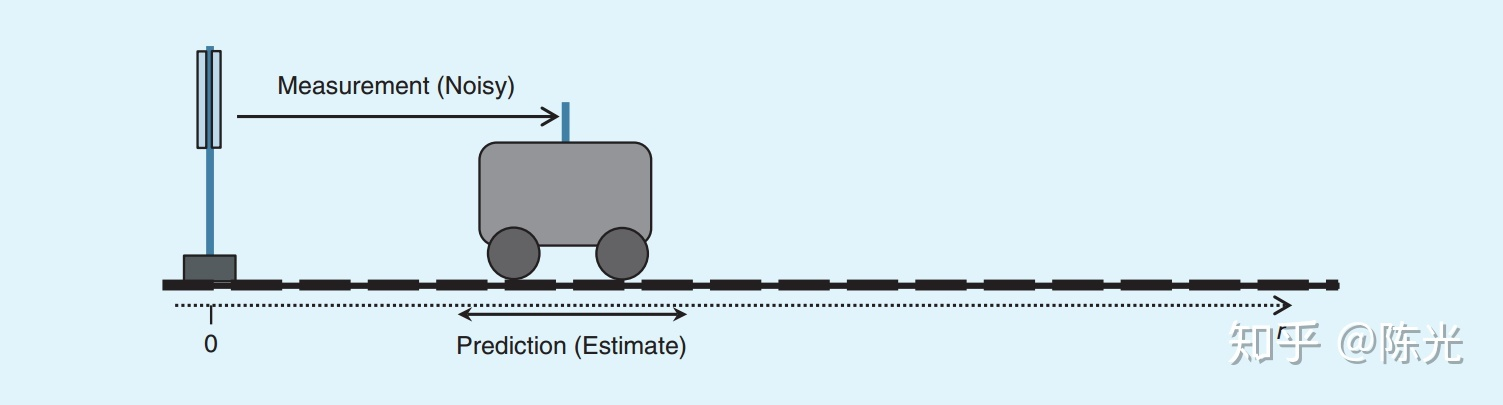
Assume that a car is moving to the right with a constant speed on the road. We installed a distance and speed sensor on the left side to measure the position s and speed v of the car once every 1 second, as shown in the figure below.
We use vector xt to represent the current state of the car, which is also the final output result, called the state vector:
Due to measurement errors, the sensor cannot directly obtain the true value of the car position, and can only obtain an approximate value near the true value, assuming that the measurement value approximately follows Gaussian distribution near the true value. As shown in the figure below, the measurement values are distributed to the left or right of the red region, and the true value is at the peak of the red region.
Since it is the first measurement, we have no historical information about the car. We assume that the state x of the car at 1 second is equal to the measurement value z, as shown below:Prediction
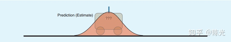
Prediction is an important step in Kalman filter, which is equivalent to predicting the future position based on historical information. Based on the position and velocity of the car in the first second, we can predict that the position of the car in the second second should be as shown in the figure below. It can be found that the range of the red area in the figure increases, which is a process of amplifying uncertainty by adding velocity estimation noise during prediction.
Based on the state of the car in the first second, the predicted state xpre can be obtained:
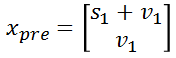
Where pre is short for prediction, the time interval is 1 second, so the predicted position is distance + velocity * 1, and the velocity remains unchanged because the car is moving at a constant speed.
Measurement
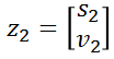
At the second second, the sensor made an observation of the position of the car. We consider that the observation value of the car at the second second is z2. The observation result of the second second is represented as a vector:
Obviously, the result of the second observation also has errors. We can see the predicted position of the car and the actual observed position of the car in the same graph as follows:
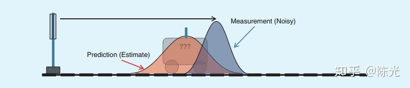
The red area in the figure is the predicted position of the car, and the blue area is the observation result of the second second.
Obviously, both of these results are near the true value. To get the result as close to the true value as possible, we weight the results of these two areas and take the weighted value as the state vector of the second second.
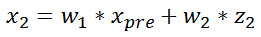
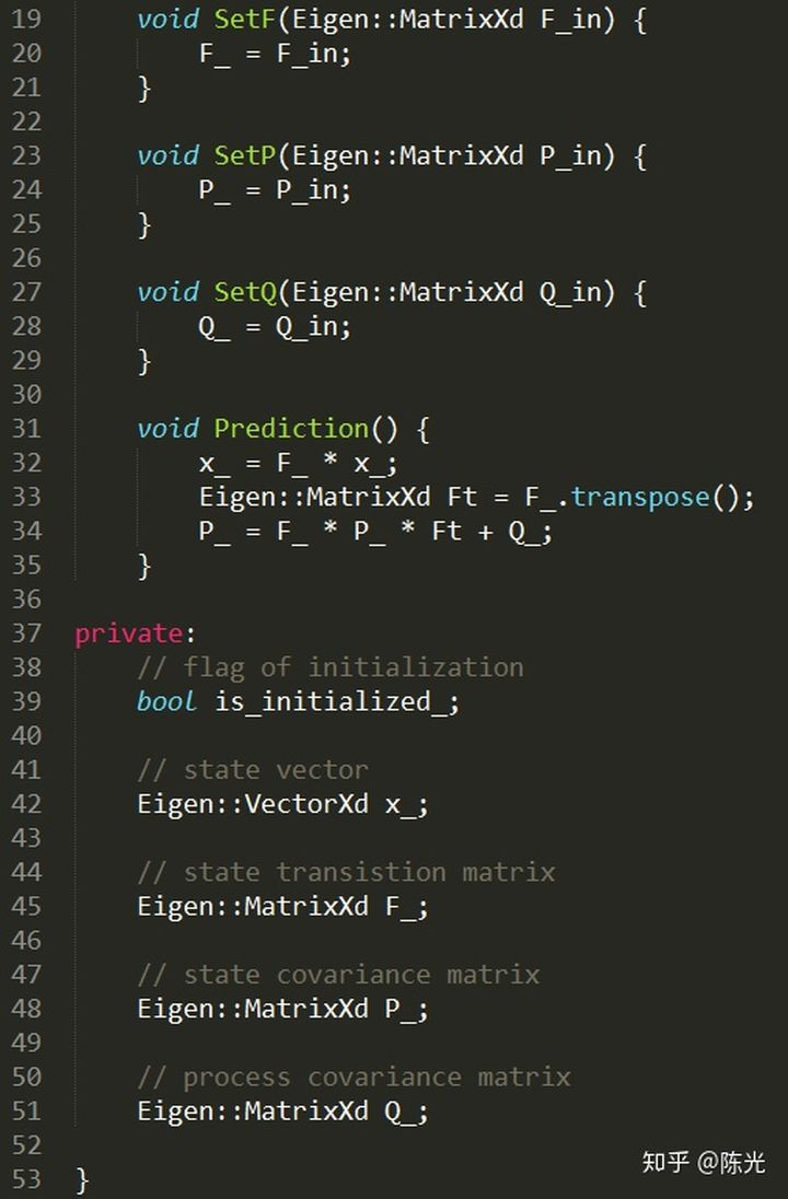
For convenience, the state vector of the second second can be written as follows:
 ## Translated English Markdown text with HTML tags preserved:
w1 and w2 are the weights for the predicted and observed results, respectively. The calculation of these weights is based on the uncertainty of the predicted and observed results, which is the variance in the Gaussian distribution. The larger the variance, the wider the wave distribution, and the higher the uncertainty. As a result, the weights given will be lower.
The distribution of the weighted state vector can be represented by the green region in the following figure, where the variance of the green region is smaller than that of the red and blue regions. This is because when performing the weighted operation, we need to multiply two Gaussian distributions to obtain a new Gaussian distribution with a smaller variance than the two Gaussian distributions that were multiplied.
Two less certain distributions are ultimately combined to form a more certain distribution, which is why the Kalman filter is highly regarded.
Prediction and Measurement
Initialization for the first second, as well as prediction and measurement for the second second, comprise one cycle of the Kalman filter.
Similarly, we make a prediction for the third second based on the state vector of the second second, and then combine it with the measurement results of the third second to obtain the state vector for the third second. We then use the state vector of the third second to make a prediction for the fourth second, and then combine it with the measurement results of the fourth second to obtain the state vector of the fourth second. We repeat this process to create a true Kalman filter.
The above is the intuitive process of the Kalman filter, and now let’s talk about how to write the above process into code.
The Theory of Kalman Filters
In the previous section, we used a simple example to introduce the entire process of the Kalman filter. In this section, we will write code to track continuous laser radar points based on the principles of the Kalman filter.
Now, we will use the valuable treasure left by Mr. Kalman himself. The following seven equations are a rational description of the Kalman filter. Using these seven equations, we can implement a complete Kalman filter. If you don’t understand these seven equations now, don’t worry, I will explain them one by one below.
Writing code (in C++) is actually the process of combining the above equations to complete the initialization, prediction, and measurement steps. Since the equations involve a large number of matrix transpositions and inverse operations, we use the open-source matrix operation library – Eigen library.
Code: Initialization# Initialization
In the Initialization step, it is necessary to initialize various variables. For different motion models, the state vector must be different. For example, in the previous example of a car, only a distance s and a velocity v are needed to represent the state of the car. In another example of a point in a 2D space, the state equation has 4 variables: the distance and velocity in the x direction, and the distance and velocity in the y direction. Therefore, we use the non-fixed-length data structure in the Eigen library. The VectorXd shown in the figure below represents a column matrix of X dimensions, and the element data type is double.
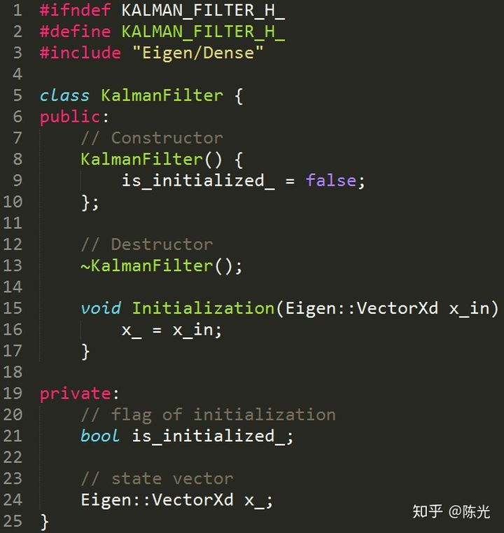
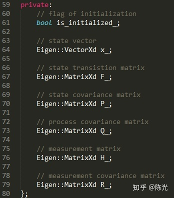
Here, we create a KalmanFilter class, which defines a variable called x_, representing the state vector of this Kalman filter.
Code: Prediction
After initialization, we begin writing the code for the Prediction section. First is the formula
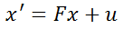
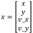
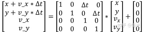
Here, x is the state vector, and the predicted state vector x' is obtained by left-multiplying a matrix F and adding external influence u. F is called the state transition matrix. Taking 2D uniform motion as an example, x is
For uniform motion, according to the formula s1 = s0 + vt from high school physics textbooks, the predicted state vector after time △t should be
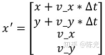
Assuming the current motion is uniform, the acceleration is 0 and will not affect the prediction, i.e.

If we use an acceleration or deceleration motion model, we can introduce the acceleration a_x and a_y, and u will become:Translate the Markdown Chinese text below into English Markdown text in a professional manner, keeping the HTML tags inside Markdown and only outputting the results.
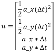
As an introductory course, we do not discuss too complex models, so the formula can be written as:

which will eventually be written as:
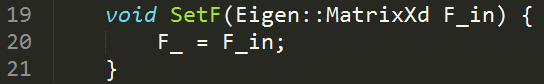
Since the size of △t is not fixed each time a prediction is made, we specifically write a function SetF()
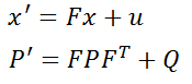
Looking at the second formula of the prediction module:
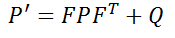
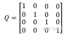
P represents the system’s uncertainty, which is large when the Kalman filter is initialized. As more and more data is injected into the filter, the uncertainty gradually decreases. The professional term for P is state covariance matrix. Q in this formula represents process noise covariance matrix, which is noise that cannot be represented by x’ = Fx + u, such as suddenly driving uphill during vehicle motion which cannot be estimated by the previous state transition.
Taking laser radar as an example, laser radar can only measure the position of points, not their velocity. Therefore, for the covariance matrix of laser radar, the measurement position is more accurate and has lower uncertainty, while the velocity information has higher uncertainty. Therefore, P can be considered as:
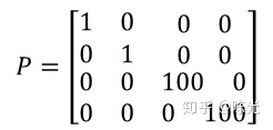
Since Q has an impact on the entire system, but it is not too certain how much impact it has on the system. In engineering, we generally set Q as the unit matrix for operation, that is:
Based on the content and formulas above:
we can now write the prediction module’s code.Translate the Chinese text below into English Markdown text in a professional manner, preserving the HTML tags inside Markdown, and output the results only, focusing on corrections and improvements without explanations.
In actual programming, x’ and P’ do not need to apply for new memory storage, and the original x and P can be used instead.
Code: Measurement
The first equation for the measurement is
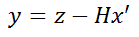
This equation calculates the difference y between the actual measured value z and the predicted value x’. The measured values of different sensors are generally different. For example, the position signal measured by lidar is the distance on the x and y axes, while the millimeter wave radar measures both position and angle information. Therefore, a matrix H, known as a measurement matrix, needs to be left multiplied by the state vector to perform corresponding operations with the measurement values.
The measured values of the lidar are
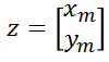
where xm and ym represent the measurements on the x-axis and y-axis, respectively.
Since x’ is a 41 column vector, in order to perform subtraction operations with a 21 column vector z, a 2*4 matrix needs to be left multiplied. Therefore, the whole equation should be written as follows:
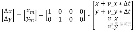
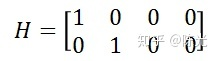
That is, for the lidar, the measurement matrix H is
After obtaining the value of y, multiply it by a weighting factor and add it to the original predicted value. This way, a state vector for the location that takes into account the measurement values and the predictive model can be obtained.
So, how should the weight of y be determined?
Let’s take a look at the next two equations:
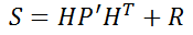
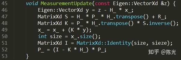
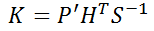 The two equations below calculate a very important parameter in the Kalman filter – the Kalman Gain K, which is the weighting of y value in layman’s terms. The R in the first equation is the measurement covariance matrix, which represents the difference between the measured value and the true value. Generally, the sensor manufacturer provides this value. S is a temporary variable used to simplify the equation.
Consider the last two equations:
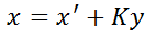
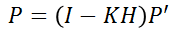
These two equations complete the closed-loop of the Kalman filter. The first equation updates the current state vector x, considering the predicted value from the last moment as well as the measurement value, and the noise of the entire system. The second equation updates the uncertainty of the system for the next cycle based on the Kalman Gain. In this equation, I is the unit matrix with the same dimension as the state vector.
The following code displays the five equations above: (Note that on line 51, “sieze” should be “size.”)
Thus, a prototype of the Kalman filter is produced.
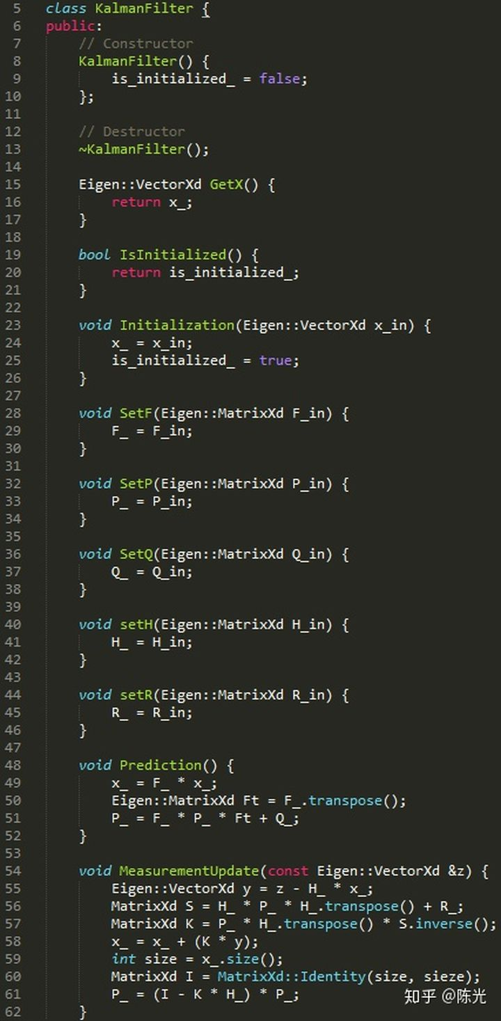
The variables contained are:
Code: Using the Kalman Filter
For example, using lidar data and the filter described above, the code is as follows (a new line containing “continue;” should be added between lines 38 and 39):
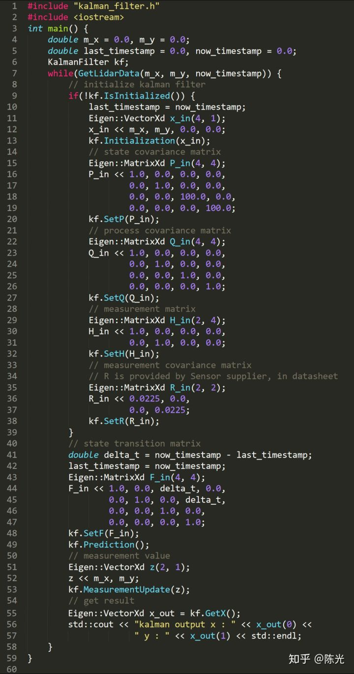
The GetLidarData function not only obtains the point position information mx and my, but also the current time stamp, which is used to calculate the time difference delta_t between the front and back frames.Below is an example of using Kalman filter to track uniformly moving objects. In addition to the classic Kalman filter, there are also extended Kalman filter and unscented Kalman filter in the industry. The biggest difference between them and the classic Kalman filter lies in the differences in the state transition matrix F and the measurement matrix H. The remaining tracking process still requires the use of the seven formulas introduced earlier.
As long as you can write the F, P, Q, H and R matrices for a certain model, any state tracking problem will be easily solved.
Conclusion
The above is the process of Kalman filter from intuition analysis to rational analysis. You will find that in real engineering development, in addition to basic coding skills, the ability to deduce formulas using linear algebra knowledge learned in university is also essential.
Ok (^o^)/~, it took me a long time to finish writing and sharing about the Kalman filter.
This article is a translation by ChatGPT of a Chinese report from 42HOW. If you have any questions about it, please email bd@42how.com.