
Author: Engineer from the Witch’s Tower
Self-attention in Transformers and cross-attention in BEV perception are two widely researched attention mechanisms. In this second article of the series, we will discuss self-attention first, and cross-attention will be introduced in the following article.
The self-attention mechanism in Transformers was first successfully applied in the field of natural language processing (NLP), replacing the commonly used recurrent neural network (RNN) for sequence data processing. Later, the self-attention mechanism was quickly extended to the visual domain and also demonstrated great potential. Although images themselves are not time series data, they can be considered as sequences in space, and videos are time series data themselves. Therefore, theoretically, self-attention can also be used to process image and video data.
Similar to the application of convolutional neural networks (CNNs) in the visual domain, self-attention also originated from image classification tasks, and ViT is one of the pioneering works in this direction. Afterwards, DETR successfully applied self-attention to object detection tasks. There are many sub-tasks in computer vision besides image classification and object detection, such as semantic segmentation, depth estimation, and 3D reconstruction. It is certainly meaningful to study the applicability of self-attention to each sub-task, but a more worthy direction of research is to extract general visual features that are applicable to multiple tasks using self-attention. This is actually quite similar to using large-scale datasets (such as ImageNet) to pretrain a general backbone network in CNN and then fine-tuning with different downstream tasks using specific datasets. Swin-Transformer and Plain Vision Transformer are two representative works in this direction. We will provide a detailed introduction to all of these directions and works in this article.
In addition to cameras, lidar and millimeter-wave radars are also commonly used sensors in autonomous driving environment perception. Although self-attention mechanisms are not widely used in the visual domain, they have gradually begun to be used to process point cloud data. Therefore, this article will also introduce the current progress in this direction. In addition, the article will briefly introduce the academic community’s exploration of the effectiveness of self-attention mechanisms.
2. Transformer from the NLP domainTransformer and self-attention mechanism were first used in NLP to process sequence data. Before Transformer, the task of processing natural language sequence data was mainly completed by recurrent neural networks (RNN) and its variants. As shown below, the structure of RNN is very simple. The core idea is to merge the previous time step state ht-1 (or “memory”) with the current time step input Xt to generate the current time step state ht, and process all the data in the sequence in this pattern. Since the parameters of the network are fixed during the training phase, the structure of RNN inevitably weakens the role of historical information and cannot maintain “long-term memory”. In addition, the training process of RNN is also affected by problems such as gradient disappearance and explosion, which is not the focus of this article and will not be discussed here.
Long short-term memory network (LSTM) adds three control gates of input, output, and forget on the basis of RNN. In addition to the fixed parameters during training phase, these control gates are also influenced by the current data, and can dynamically control what information needs to be remembered and forgotten, and by how much. Through this dynamic gate control mechanism, LSTM can better maintain long-term memory, so it can handle longer sequences.
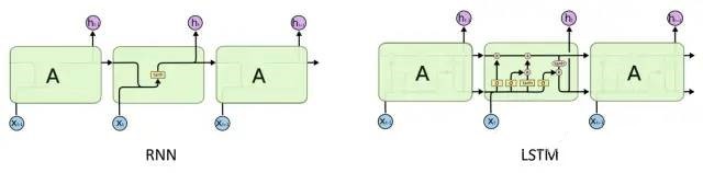
Compared with RNN, LSTM can better handle long-term dependency relationships, that is, it can extract long-term correlations. However, whether it is RNN or LSTM, processing is done sequentially. This method limits the parallel processing ability of the system on one hand, and on the other hand, sequential processing still loses information. For very long-term correlations, especially global correlations (where global refers to the entire time series), they are still powerless. In this context, Google researchers proposed the Transformer model based on self-attention mechanism in the paper “Attention is all you need” in 2017, breaking the sequential processing restriction and extending the range of correlation extraction to the global dimension. The model achieved significant performance improvements in many NLP tasks, and initiated a hot research trend on attention mechanism in the industry.# About Transfomer, you can find a lot of detailed articles on Zhihu. We won’t reinvent the wheel here, but to ensure the completeness of the article, we will introduce briefly the core idea of Transfomer.
2.1 Calculation Method of Self Attention
The core of Transfomer is self-attention, and the essence of self-attention lies in the “self” above, because it describes the correlation between each element of the data (corresponding to the Token in the paper), that is, the intrinsic relationship within the data itself. In theory, self-attention itself does not limit how to extract the correlation between data elements, but currently, everyone generally refers to the dot-product attention used in Transformer as self-attention. This is also a very common way of correlation calculation in statistics.
As shown in the above figure, the calculation in self-attention involves Query, Key, and Value, which correspond to Q, K, and V in the formula, respectively. They are all obtained by transforming the input data. For example, if the input data is a sentence containing multiple words, each word is represented by a vector. By learning three different transformation matrices for processing, each word can be transformed into the corresponding Query, Key, and Value. Multiple words are combined to form a matrix. In the attention calculation formula above, Q and K are multiplied, corresponding to the dot-product operation of Query and Key. The result is the similarity between Query and Key. Then, scaling is performed according to the dimension of the Key vector (dk). Afterwards, the softmax operation normalizes the similarity among multiple keys corresponding to a query so that their sum is equal to 1. These similarities serve as weights to perform weighted average on the corresponding value, and the output corresponding to this query is finally obtained. This whole process is actually the process of encoding or feature extraction of the input data, and the basis of encoding is the correlation between the internal elements of the data.
To enhance the capability of information extraction, the encoding process described above can be repeated in parallel multiple times, and the results of multiple encodings are overlapped to obtain the final output. This structure is called multi-head attention, which is essentially a combination of multiple single-head attentions.
In terms of computational complexity, the computational complexity of self-attention is O(N²), where N represents the number of input elements, such as the number of words in a sentence. In the next section on visual attention, we will see that this quadratic calculation complexity will lead to poorer scalability of the algorithm on high-resolution images.
2.2 Design Motivation of Self-Attention
The above is the core part of self-attention calculation, which is not complicated and can be easily understood and reproduced from both the original paper and various interpretive articles. However, what is the design motivation behind this process? Because we will introduce the application of self-attention in visual perception later, let’s explain it with visual tasks as an example here.
As we mentioned before, the task of self-attention is to encode the input data, which is to extract features. So, let us recall the classic feature extraction methods in computer vision. Before deep learning became popular, we usually manually designed some feature extraction templates, such as SIFT, Gabor, HOG, etc. These features describe the characteristics of local areas in the image and have good invariance to some changes such as scale, lighting, etc. Of course, there are also some global features, such as using Fourier transform to extract low-frequency signals from images, but they are not commonly used. After deep learning dominates the visual field, we generally use convolution operations to extract local image features, and the convolutional kernel is obtained through training.
Whether it is global features or local features, whether it is hand-designed or deep learning, the essence of feature extraction is to describe the correlation of data itself. For example, a 3×3 convolution kernel describes the relationship between the central pixel and the surrounding 3×3 neighborhood. However, the scope of these feature extraction methods is fixed, and the extraction template is also fixed. Local features extract information within a fixed size region, and larger scopes are usually obtained by scaling images or stacking feature extraction layers. Global features can describe the entire image, but they are usually more general descriptions that lose detailed local information.
From the computation of self-attention, we can see that the feature extraction of each element uses all elements in the data. Therefore, theoretically, this is a kind of global feature extraction. However, this global feature extraction uses a weighted sum method, and the weight is the correlation between elements, which is dynamically calculated. That is to say, elements with low correlation will have a relatively small effect in the feature extraction process. This makes the feature extraction process have a certain focus and will not lose important local information. Therefore, the self-attention mechanism can simultaneously take into account the global and local aspects of feature extraction and self-determine the focus of feature extraction through data and task-driven methods.2.3 The Network Architecture of Transformer
As shown in the figure below, Transformer is an encoder-decoder structure, consisting of six encoders and six decoders (N=6). Here we will briefly introduce its workflow.
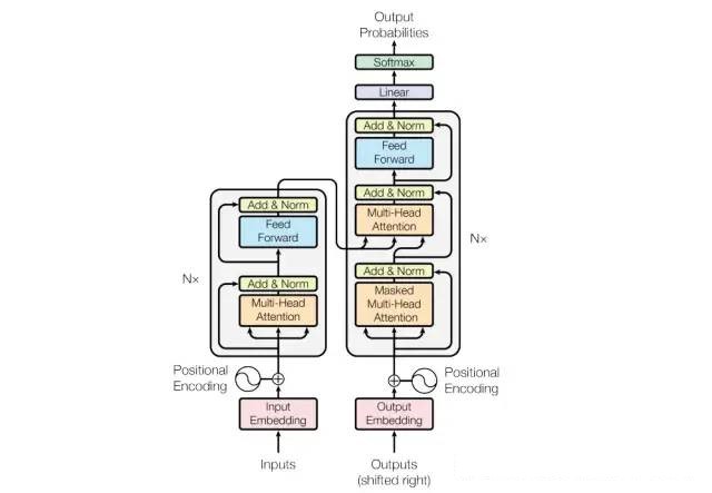
Firstly, each element in the input data needs to go through a feature extraction process. This step is mainly related to the specific task, for example, converting words into word vectors, or converting image blocks into pixel vectors. Assuming that the input data contains M elements and the feature vector dimension of each element is d, then the dimension of the input data is M*d.
The calculation of self-attention does not consider the positional information of the elements, but this information is usually important for subsequent tasks. Therefore, Transformer adds the position encoding feature to the input features. The calculation formula of position encoding is shown below. The position feature generated by this formula has the same dimension as the input feature d. After adding with the input feature, it can be used as the input of the encoder. Its dimension is also Mxd.

The encoder is mainly composed of two parts: multi-head attention and fully connected layer (Feed Forward). Both parts include residual connection (Add) and normalization (Norm). These two operations are commonly used techniques in deep learning, so we will not elaborate on them. Multi-head attention was detailedly introduced in the previous section, and the fully connected layer is used for further feature extraction of the encoded elements, but it does not involve the relationships between the elements. Each element is operated independently. After these operations, the output dimension is still Mxd, but at this point, the feature of each element contains all the relevant information of other elements. The multi-head attention and the fully connected layer are repeated six times as a module in the encoder to extract higher-level features with more semantic information.In NLP tasks, the decoder is also a very important step. For example, in the sentence translation task, after the input sentence generates features through the encoder, it also needs to be input to the decoder to obtain the translated sentence. The structure of the decoder is very similar to the encoder, both are multi-head attention plus fully connected layers, repeated six times. The main differences between the decoding and encoding processes are the following two points.
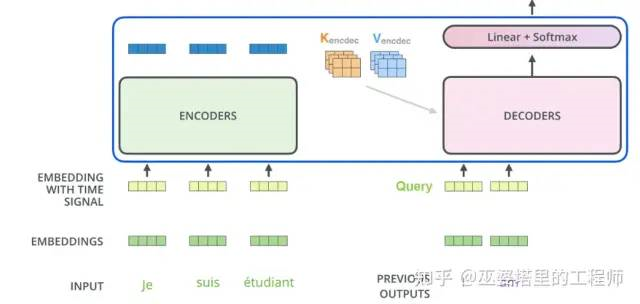
First, the decoder has two inputs. One is the output of the encoder, which is processed as key and value, and the other is the feature of the current word to be decoded after being processed by the multi-head attention module, which serves as the query. Therefore, this is a cross-attention between encoding and decoding, where the query comes from the decoder and the key and value come from the encoder. During the decoding process, the key and value remain unchanged.
In addition, during the training process, in order to prevent the network from using elements that have not yet been decoded, a mask is needed to cover these elements, and in the prediction process, the initial decoding results will be set to empty.
3. Self-Attention in Visual Perception
Similar to Convolutional Neural Networks (CNNs), self-attention mechanisms in visual perception also started with the relatively simple task of image classification. Afterwards, self-attention was successfully extended to the field of object detection. Recently, self-attention has been applied to backbone network structures to support various downstream visual perception tasks. The following will introduce the application of self-attention in visual perception according to this development thread.
3.1 Image Classification
Vision Transformer (ViT) is the first successful application of Transformers in the field of image classification. The core idea is to divide the two-dimensional image into multiple equally-sized image blocks. If the image is regarded as a “sentence” in NLP, then the image blocks can be regarded as “words” or tokens. With this representation structure, the Transformer encoder in NLP can be directly used to extract image features. The idea of ViT is intuitive, but there are several details to note in the specific implementation process.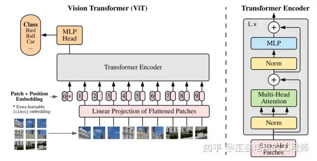
Class embedding vector. Transformer encoder extracts features from multiple image patches, but what features should be used to complete image classification? A simple method is to merge the features of all image patches, for example, using MeanPooling. In ViT, an additional class embedding vector is used, which, like the image patch, participates in the encoding process as a token. Therefore, this vector will eventually contain information about all image patches. According to the calculation method of self-attention introduced in Section 2.1, this vector is actually the weighted average of the features of all image blocks, and the weight is obtained by learning. The class embedding vector is finally connected to the MLP Head to complete the image classification task.
Position encoding. The original Transformer used fixed position encoding features, while ViT uses a learnable 1D position encoding feature. Each image block has its own position feature, which can be optimized during training. ViT also tested 2D position features and relative position features, but did not obtain better results. Regardless of which type of position encoding feature is used, its function is to distinguish the position of image blocks. The position features of each image block are different, which also ensures that the order of image blocks cannot be arbitrarily distorted when inputting.
Pre-training. The ViT model based on Transformer can only demonstrate its advantages over CNN networks when pre-trained on large datasets (such as JFT with 300M images). On small datasets, the accuracy of the two is similar. In addition, ViT can use the feature map processed by CNN instead of the original image as input, that is, combining CNN and Transformer. This method has significant advantages on small datasets, and is comparable to the performance of Transformer when trained on large datasets.
3.2 Object Detection
With the successful application of ViT in image classification tasks, Transformer has also begun to show its strength in the field of object detection. DETR is the earliest and most representative work in this regard.3.2.1 DETR
The network structure of DETR can be mainly divided into three parts: CNN backbone, encoding-decoding network, and feedforward prediction network.
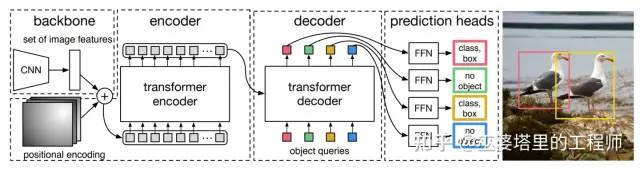
DETR uses a CNN backbone network to extract basic image features, and the width and height of the feature map are 1/32 of the original image. In other words, each point on the feature map corresponds to a 32×32 area in the original image. This method is similar to the way of dividing the image blocks in ViT, and is a mixed method of CNN and Transformer. As mentioned in the last section, this mixed feature extraction method has obvious advantages on small datasets.
Based on the image block partition, DETR can use the same encoder structure as ViT. The only difference is that DETR uses a fixed position encoding feature. As for the decoder, ViT does not have this module, and DETR uses a combination of encoding-decoding attention and self-attention, which is the same as Transformer. Specifically, the key and value come from the output of the encoder, and the query is processed using self-attention. The difference between DETR and Transformer lies in the source of the query and the decoding method. The query in Transformer is the word to be decoded, and the decoding process is sequential. That is to say, the query is inputted one by one according to the order of the words in the sentence. The decoding process of DETR is parallel, and N queries are inputted to the decoder at the same time. Here, N represents the maximum number of targets, which can be thought of as N words in the dictionary, and the query is actually the embedding of these N words. The function of these embeddings is similar to the position encoding. The position encoding is used to distinguish different positions of image blocks, while the embeddings are used to distinguish different target objects.
The decoder outputs N feature vectors, and after processing by the feedforward network, information of N targets, including category and object boundary, can be obtained. Here, the category can be “background”, which means there is no target. Therefore, the object detection task is completed. From this process, it can be seen that the detection of each target uses information from all positions on the image, so this is a object detection method based on the global receptive field.The DETR outputs a set of targets, so the loss function during training needs to be able to measure the similarity between the output set and the annotated set. This is a bipartite matching problem, and DETR uses the Hungarian algorithm to calculate the optimal match and provides the corresponding matching loss. This article mainly focuses on the attention mechanism, so this part will not be elaborated on.
Thanks to the global receptive field, DETR has relatively high accuracy in detecting large objects, but the detection effect of small objects is not satisfactory. This is mainly because the CNN backbone network significantly reduces the resolution of the image, and low-resolution feature maps lose a lot of information, which is especially serious for small objects. Increasing the resolution of the feature map can improve the detection effect of small objects, but it will greatly increase the computation of the encoder and decoder (the computation is proportional to the square of the number of image blocks). In addition, the convergence speed of DETR during training is very slow, only about one-tenth to one-twentieth of Faster RCNN. This is mainly because in the calculation of self-attention, the image blocks are fully connected, and the weights of the connections are initially evenly distributed. The learning process requires reweighting these connections. From the final learning results, only a few connections are retained, that is, the connection changes from dense to sparse.
The two problems of large computation caused by increasing the resolution and slow training convergence are both caused by the dense connectivity of image blocks, or the global receptive field. In the object detection task, the global receptive field can better model contextual information, but the key information for detection still comes from the region around the object. Since it is not cost-effective to spend a lot of computation and training time to model the global receptive field, people naturally think of directly constructing sparse attention instead of learning it through laborious efforts. There are many ways to construct sparse attention, such as limiting attention calculation to manually defined local areas, or using deformable convolutions to allow the network to automatically learn where to calculate attention from sparse positions. The following introduces Deformable DETR, which uses the latter to sparsify attention calculation, thereby reducing computation and accelerating training.
3.2.2 Deformable DETR
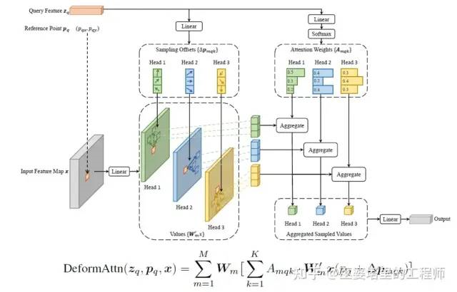
Deformable DETR has the same basic structure as DETR, and the main difference is in the details of attention calculation. The former only calculates attention on a fixed number of keys, while the latter corresponds to all image blocks, or each position of the feature map.
In the example below, the number of keys is fixed at 3, denoted by K=3. Each position on the feature map can serve as a query, represented by its feature
and its location
. The position of the key relative to the query
(i.e., which sparse positions to calculate the attention from) and the attention weight
are learned. The position of the key comes from the query feature
, the value of the key comes from the corresponding position on the feature map
, and the attention weight also comes from the query feature
. This is different from the traditional usage of query, key, and value in self-attention calculations. Moreover,
corresponds to multi-head attention in the following formula. By using this sparse approach, the complexity of attention calculation is reduced to
, where
refers to the size of the feature map.
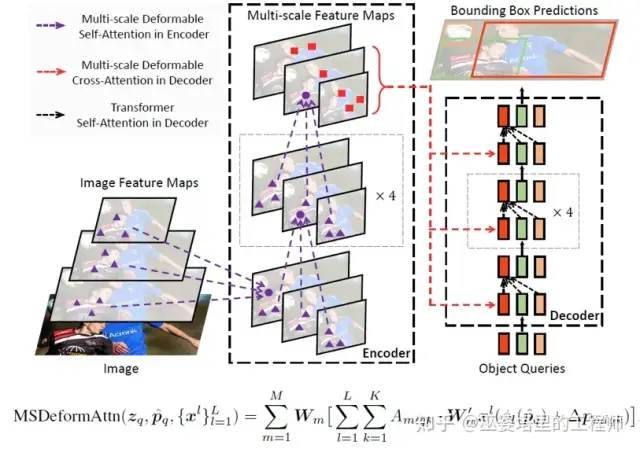
To obtain information with multiple resolutions, deformable attention can also be computed on feature maps with multiple resolutions. The output of the final encoder is still a feature map with multiple resolutions, but the feature of each position on the feature map encodes information from various resolutions. The decoding process is similar to that of DETR, except that deformable attention is used in the cross-attention phase. In this phase, the position
corresponding to object queries is obtained by linearly transforming query embeddings.
3.3 Backbone Network
The application of attention to image classification and object detection tasks involves two stages: encoding and decoding. The decoding stage in image classification can be regarded as being implicit in the category embedding vector. The encoder is used to extract image features, and the decoder corresponds to downstream tasks. If we only consider the encoder, then the role of attention mechanism here is to extract better image features, which is similar to the role of CNN as the backbone network. Therefore, the Transformer can also be used as the backbone network to support various downstream tasks. In fact, in the experiments of DETR, the author has tried to use the feature map generated by the encoder for panoramic segmentation task and achieved good results. The multi-resolution feature map generated by the encoder in Deformable DETR can also be regarded as a feature pyramid used for various downstream tasks.Using Transformer as the backbone network has become a trend in attention research. In order to adapt to various downstream tasks, the backbone network needs to output feature maps of different resolutions, especially high-resolution feature maps. However, the computational cost of self-attention is proportional to the square of the image size, and computing self-attention on high-resolution images requires very high hardware computing power. Therefore, the main focus of research in this area is to solve the conflict between resolution and computational complexity.
Deformable DETR adopts the idea of deformable convolution, which limits the calculation of attention to a limited number of pixels (usually far less than the size of the image). In addition, there are two other typical works: Swin-Transformer and Plain Vision Transformer.
3.3.1 Swin-Transformer
The core idea of Swin-Transformer includes two points: multi-resolution feature extraction and Transformer module based on shifted window (Swin).
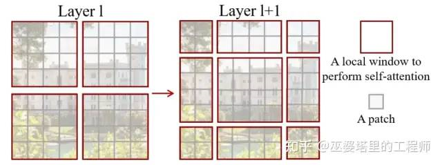
The structure of multi-resolution feature extraction is shown in Figure a below. The basic processing unit token is a 4×4 pixel RGB image block, so the input size of the network is H/4 x W/4 x (4x4x3). In Stage 1, after linear feature extraction and two Swin modules, the resolution remains unchanged, but the feature dimension becomes C. In Stages 2/3/4, adjacent 2×2 image blocks are merged, the resolution is reduced to 1/2 of the original, and the feature dimension is originally 4 times the original, but finally reduced to 2 times. Through the above operations, multi-resolution feature maps can be obtained, with resolutions of 1/4, 1/8, 1/16, and 1/32 of the original image, and feature dimensions of C, 2C, 4C, and 8C, respectively.
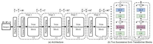
In the Transformer module based on window offsets, the computation of multi-head self-attention (MSA) is performed in local windows instead of the entire image. As shown in the example in the figure below, the computation of self-attention is first performed in non-overlapping windows of 4×4 image blocks (Layer 1, W-MSA), and then the window is horizontally and vertically shifted by 1/2 window size, which is 2 image blocks. Self-attention calculation is then performed inside the shifted window (Layer 2, SW-MSA). W-MSA and SW-MSA together form a Swin Transformer module (figure b), which is repeated twice in feature extraction for each resolution. Limiting attention calculation to local windows ensures that its computational cost is linearly proportional to image size, greatly reducing the overall computational burden in high-resolution cases. Alternating different forms of window partitioning increases information flow between windows, thereby increasing the spatial coverage of attention calculation and expanding the receptive field. Therefore, this method of attention calculation can achieve a good balance between resolution, computational cost, and receptive field.
In addition, it is worth mentioning that when calculating the similarity between the query and key in Swin Transformer, the positional differences of the corresponding image blocks are also taken into account. Experimental results have shown that this method is more effective than traditional positional encoding.
Swin Transformer can replace traditional CNN backbone networks in three common visual tasks: image classification, object detection, and semantic segmentation, with comparable or even lower computational costs, while achieving significant improvements in accuracy. The improvement in accuracy is not surprising, as self-attention has stronger feature extraction capabilities than convolutional networks. The reduction in computational cost is mainly attributed to limiting attention calculation to local windows, but this is at the cost of sacrificing feature extraction capabilities. The window offset mechanism allows information to flow between windows, expanding the receptive field of feature extraction to a certain extent, thus mitigating the impact of local window limitations. This is also the key to the success of Swin Transformer.3.3.2 Plain Vision Transformer (PlainViT)
In object detection and semantic segmentation networks, pyramid-structured backbone networks (such as FPN) are usually important components. The pyramid structure can help extract multi-scale features, thereby enabling better perception of objects of different sizes. However, the pyramid structure is designed for downstream tasks, which requires training on specific datasets (such as COCO, KITTI, etc.). This makes it difficult for the backbone network to be pre-trained on large-scale datasets (such as ImageNet), while pre-training on large datasets is usually the basis for successful attention mechanisms.
How to solve this dilemma? The idea proposed by Plain ViT is to use a single-scale backbone network and multi-scale detection heads. The backbone network can be pre-trained on large-scale datasets, while the detection head is trained only on the corresponding specific task dataset. This can separate upstream and downstream tasks, making the system more modular and adaptable, but the premise is that the backbone network can also learn scale-invariant features.
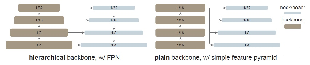
As shown in the figure above (right), PlainViT uses a single-scale backbone, and the patch size is set to 16×16, so the resolution of the feature map is 1/16 of the original image. This is consistent with the patch size of ViT, so the backbone of ViT can be directly used, which is also the biggest motivation for the design of PlainViT. Object detection and semantic segmentation networks require high-resolution inputs, so PlainViT also uses windowed attention similar to Swin-Transformer to reduce computational cost. The window size here is consistent with the feature map size (number of patches) of ViT, which is 14×14. Of course, this is also to better utilize ViT’s backbone network.Translate into English Markdown text, preserving HTML tags inside Markdown in a professional manner, outputting only corrections and improvements.
The window attention loses global information, and Swin-Transformer uses window shifting mechanism to ensure information exchange between different windows. PlainViT experiments with two different strategies. The first is the standard global attention, and the second adds one or more residual convolution modules after window attention. Both strategies promote information flow between windows, but inevitably increase computational load. Therefore, in PlainViT, the backbone network is divided into four groups, each with six attention blocks, and **the above two window information exchange strategies are only implemented in the last block of each group to ensure that the computational load does not increase too much.

PlanViT's backbone network is single-scale, but the detection head obtains multi-resolution feature maps through upsampling and downsampling to complete downstream tasks. Experiments have shown that this simple sampling is very effective and shortcut connections similar to FPN are not necessary. The authors believe that this is due to the spatial detail information preserved by the position encoding and high-dimensional patch feature encoding in ViT, which allows direct upsampling to restore high-resolution signals.

PlanViT provides many comparative experimental results in the article, which will not be listed one by one. The most important conclusion is that by using Masked AutoEncoder (MAE) for unsupervised pre-training, PlainViT outperforms Swin-Transformer, which is based on a multi-scale backbone network, especially with larger backbone network size, on COCO dataset.

### 4. Self-Attention in Point Cloud Processing

After achieving success in the field of computer vision, the self-attention mechanism has also been naturally applied to point cloud processing. In these applications, the core algorithm of self-attention remains the same, but the data being processed is different. Therefore, this article only gives an overview of how to process point cloud data, without going into details about specific methods.

Unlike images, point clouds are unstructured data. Generally speaking, point cloud data can be represented as point views and grid views. For this, you can refer to the introduction to point cloud object detection in this column.

If the point view is used, that is, processing the original point directly, we can treat each point in the point cloud as a token, and the self-attention mechanism can be applied smoothly to point cloud data. At this time, all points in the point cloud will affect each other, that is, global attention is extracted. Although this method can obtain the maximum receptive field, the computational load will also increase sharply when the point cloud size is large, which is similar to the problem faced in the field of computer vision. Therefore, some researchers propose to use local attention, and use a hierarchical clustering method similar to PointNet++ to hierarchically cluster the point cloud, so that the attention calculation is limited to the local clustering of each layer. Such an approach can effectively reduce the computational load, and hierarchical clustering can ensure that both local and global information is extracted. This is similar to the principle of Swin-Transformer introduced earlier.
If we adopt grid view, i.e. convert point cloud into grid form in advance, then it is very similar to image format, and self-attention methods in the visual field can theoretically be directly used. Of course, the grid data here is relatively sparse, and the sparse convolution commonly used in grid processing can also be applied to the calculation of self-attention in order to improve computational efficiency.
5. Discussion on Self-Attention Mechanism
Transformer and self-attention mechanism have achieved great success in the visual field in recent years. What is the fundamental reason behind this? Is it the way of calculating relevance, global perception, or dynamic attention calculation? This is a very meaningful topic, and some researchers have recently started to try in this direction. One typical work is MLP-Mixer.
The structure of MLP-Mixer is very simple. First, similar to ViT, the input image is divided into small blocks and preliminary feature extraction is performed using fully connected layers. In this way, each image block has its own features and can be viewed as a token. Next is the core Mixer layer, which includes two steps: Token-mixing and Channel-mixing. The former operates on the Token level, which is actually to use MLP for weighted averaging of all Tokens. This is similar to the weighted averaging in self-attention, but the weights provided by MLP are not directly related to the correlation between Tokens, and are fixed in the training stage rather than dynamic. The latter is just a standard fully connected layer used to extend the channel/feature dimension.
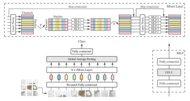
Compared with ViT, MLP-Mixer has no relevance calculation or dynamic attention, and the only thing retained is the global perception (Token-mixing layer). However, in image classification tasks, MLP-Mixer can achieve similar effects as ViT, especially under the premise of massive training data and ultra-large network scale. This research result shows that the success of Transformer mainly comes from two points: global perception and massive training data. As for the calculation method of self-attention, at least from the comparison with MLP-Mixer, it is not particularly important. Of course, this is just a result of a work, and more researchers need to explore this direction in depth in the future.# 这是一个Markdown示例文本
这是一个包含粗体、斜体和代码块的示例文本。还有一个链接和一个图片。

<!-- 这是一个HTML代码块 -->
<div class="example">
  <p>Hello, world!</p>
</div>
以上是示例文本。
This article is a translation by ChatGPT of a Chinese report from 42HOW. If you have any questions about it, please email bd@42how.com.