Foreword

For autonomous driving applications, perception of 3D scenes is ultimately required. The reason is simple: vehicles cannot rely on perceiving results from a single 2D image to drive, and even human drivers cannot drive just by looking at an image. This is because the distances and depth information of objects cannot be reflected in 2D perception, while these information are crucial to make correct judgments for the autonomous driving system regarding the surrounding environment.
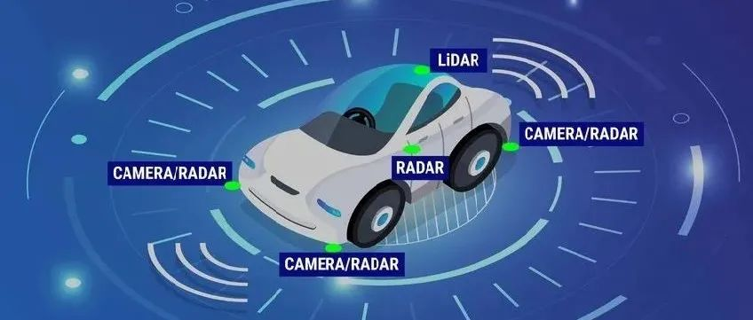
In general, the visual sensors (such as cameras) of autonomous driving vehicles are installed either on the top of the body or on the rearview mirror inside the vehicle. Regardless of the position, what the camera obtains is the projection of the real world in the perspective view (from the world coordinate system to the image coordinate system). This view is similar to the human visual system, so it is easy for a human driver to understand. However, the perspective view has a fatal flaw, which is that the scale of objects varies with distance. Therefore, when the perception system detects an obstacle ahead in the image, it does not know the distance between this obstacle and the vehicle, nor does it know the actual three-dimensional shape and size of the obstacle.
!Image coordinate system (perspective view) vs. World coordinate system (bird’s eye view) [IPM-BEV]
![Image coordinate system (perspective view) vs. World coordinate system (bird’s eye view) [IPM-BEV]](https://upload.42how.com/article/image_20220114004846.png)
To obtain information about 3D space directly, the most direct method is to use a lidar. On the one hand, the 3D point cloud output by the lidar can be directly used to obtain the distance and size of obstacles (3D object detection), as well as the depth of the scene (3D semantic segmentation). On the other hand, the 3D point cloud can also be fused with the 2D image to make full use of the different information provided by the two: the advantage of point clouds is that they provide accurate distance and depth perception, while the advantage of images lies in richer semantic information.
However, the lidar also has its drawbacks, such as high cost, difficulty in mass production of vehicle-grade products, and greater susceptibility to weather conditions, etc. Therefore, 3D perception based solely on cameras is still a very meaningful and valuable research direction. The following parts of this article will detail the 3D perception algorithms based on single and dual cameras.
Single-Camera 3D Perception
Using a single camera image to perceive a 3D environment is an ill-posed problem, but some geometric constraints and prior knowledge can be used to assist in completing this task. One can also learn through end-to-end deep neural network how to predict the 3D information from image features.
Object Detection
Image Inverse Perspective Mapping (IPM)
As mentioned earlier, images are projections from the 3D world onto a 2D plane. Therefore, a direct solution for 3D object detection from image is to inverse project the 2D image back into the 3D world, followed by object detection in the world coordinate system. This is theoretically an ill-posed problem, but it can be tackled with additional information such as depth estimation or geometric assumptions such as pixel lie on the ground plane.
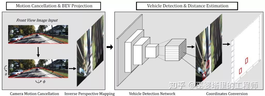
BEV-IPM [1] proposed to transform the image from the perspective view to a bird’s eye view (BEV). There are two assumptions involved: the first is that the ground is parallel to the world coordinate system and is at zero height. This may not hold in the case of non-flat surfaces. The second assumption is that the vehicle’s coordinate system is parallel to the world coordinate system. The latter can be corrected by the vehicle’s pose parameters (Pitch and Roll), which amounts to a calibration between the vehicle and the world coordinate systems. Assuming that all pixels in the image have zero height in the 3D world, a Homography transformation can be used to map the image into the BEV. In the BEV view, a YOLO-based method is used to detect the bottom box of the target object, which is the rectangle that touches the ground plane. The height of the bottom box is zero, and therefore it can be accurately projected onto the BEV view as ground truth for training neural networks. The predicted box by the neural networks can also accurately estimate its distance. The assumption here is that the target object needs to touch the ground, which is generally true for vehicle and pedestrian targets.
 Another method of inverse transform is the Orthographic Feature Transform (OFT) [2]. Its idea is to use CNN to extract multi-scale image features, then transform these image features to BEV view, and finally perform 3D object detection on the BEV features. First, it is necessary to construct a 3D grid under the BEV perspective (the grid range in the experiment is 80 meters x 80 meters x 4 meters, and the grid size is 0.5m). Each grid corresponds to a region on the image by perspective transformation (defined as a rectangular region for simplicity), and the mean of the image features in this region is used as the feature of the grid, thus obtaining the 3D grid feature. In order to reduce the calculation, the 3D grid feature is compressed (weighted average) in the height dimension to obtain a 2D grid feature. The final object detection is performed on the 2D grid feature. The projection from the 3D grid to the 2D image pixel is not one-to-one, and multiple grids correspond to adjacent image regions, leading to ambiguity in grid features. Therefore, it is also necessary to assume that the objects to be detected are all on the road, and the range of height is very narrow. Therefore, in the experiment, the 3D grid height is only 4 meters, which is enough to cover vehicles and pedestrians on the ground. However, if you want to detect traffic signs, this kind of method that assumes that objects are close to the ground is not applicable.
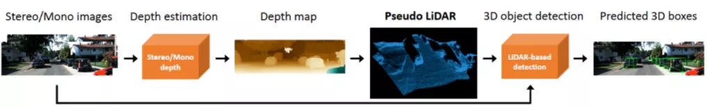
 The above two methods both assume that the object is located on the ground. In addition, another approach is to use the results of depth estimation to generate pseudo point cloud data, with one typical work being Pseudo-LiDAR [3]. The results of depth estimation are generally regarded as additional image channels (similar to RGB-D data), and image-based object detection networks are directly used to generate 3D object bounding boxes. The authors pointed out in the paper that the reason why the accuracy of 3D object detection based on depth estimation is much worse than that of LiDAR-based methods is not mainly due to the insufficient accuracy of depth estimation, but rather due to problems in the representation of data. Firstly, the area of far objects in image data is very small, which makes the detection of far objects very inaccurate. Secondly, the depth difference between adjacent pixels in depth may be very large (e.g., at the edge of an object), which will cause problems in feature extraction using convolutional operations. Considering these two points, the authors proposed to convert the input image into point cloud data similar to that generated by LiDAR based on the depth map, and then to use algorithms that combine point cloud and image fusion (such as AVOD and F-PointNet) to detect 3D objects. The Pseudo-LiDAR method does not depend on a specific depth estimation algorithm, and any depth estimation from monocular or binocular can be used directly. With this special data representation method, Pseudo-LiDAR can improve the accuracy of object detection from 22% to 74% within a range of 30 meters.
Compared with real LiDAR point clouds, the Pseudo-LiDAR method still has certain gaps in the accuracy of 3D object detection, mainly due to the insufficient accuracy of depth estimation (binocular is better than monocular), and especially the depth estimation errors around the object will have a great impact on detection. Therefore, many extensions have been made to Pseudo-LiDAR. Pseudo-LiDAR++ [4] uses a low-beam LiDAR to enhance the virtual point cloud. Pseudo-Lidar End2End [5] uses instance segmentation instead of object boxes in F-PointNet. RefinedMPL [6] only generates virtual point clouds on foreground points, reducing the number of point clouds to 10% of the original, which can effectively reduce the number of misdetected points and the computational complexity of the algorithm.
Key Points and 3D Models
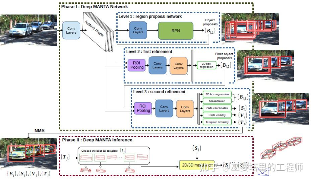
In autonomous driving applications, many targets that need to be detected (such as vehicles and pedestrians) have relatively fixed sizes and shapes, and are known in advance. This prior knowledge can be used to estimate the 3D information of the target.# DeepMANTA [7] is one of the pioneering works in this field. First, traditional image object detection algorithms such as Faster RNN are used to obtain 2D object boxes and detect keypoints of the vehicles. Then, these 2D object boxes and keypoints are matched with various 3D vehicle CAD models in the database, and the model with the highest similarity is selected as the output of 3D object detection.
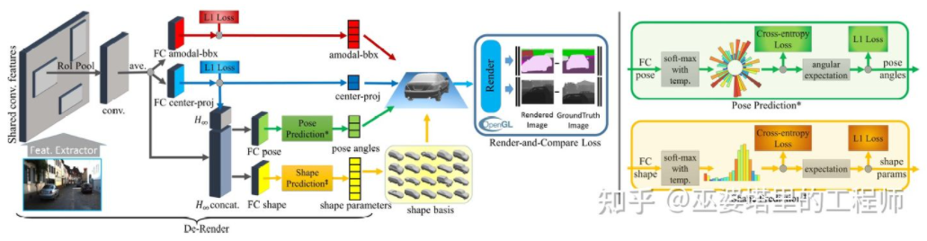
3D-RCNN [8] proposes to use the Inverse-Graphics method to recover the 3D shape and pose of each object in the scene based on the image. Its basic idea is to start from the 3D model of the object and find the model that best matches the object in the image by parameter search. These 3D models usually have many control parameters, and the search space is very large. Therefore, traditional methods are not good at searching for the optimal solution in high-dimensional parameter space. 3D-RCNN uses PCA to reduce the dimensionality of the parameter space (to 10-D), and uses deep neural networks (R-CNN) to predict the low-dimensional model parameters of each object. The predicted model parameters can be used to generate the 2D image or depth map of each object, and the Loss obtained by comparing with GroundTruth data can be used to guide the learning of the neural network. This Loss is called Render-and-Compare Loss, which is implemented based on OpenGL. The 3D-RCNN method requires a lot of input data, and the design of Loss is relatively complex, which makes the engineering implementation difficult.
 # Translation
MonoGRNet [9] proposes to divide monocular 3D object detection into four steps, each used to predict the 2D object box, the depth of the object’s 3D center, the 2D projection position of the object’s 3D center, and the 3D positions of eight corners of the object. Firstly, the predicted 2D object box in the image is used to obtain the visual features of the object through the ROIAlign operation. Then, these features are used to predict the depth of the object’s 3D center and the 2D projection position of the 3D center. With these two pieces of information, the location of the object’s 3D center point can be obtained. Finally, based on the position of the 3D center, the relative positions of the eight corners can be predicted. MonoGRNet can be regarded as using the center of the object as the key point, and the matching of 2D and 3D is calculated based on point distance. MonoGRNetV2 [10] extends the center point to multiple key points and uses 3D CAD object models for depth estimation, which is similar to the previously introduced DeepMANTA and 3D-RCNN.

Monoloco [11] mainly solves the problem of 3D detection of pedestrians. Pedestrians are non-rigid objects, and their postures and deformations are more diverse, making them more challenging than vehicle detection. Monoloco is also based on key point detection, and the relative 3D positions of prior key points can be used for depth estimation. For example, the distance from a pedestrian’s shoulders to hips, which is 50 cm, can be used to estimate the pedestrian’s distance. The reason for using this length as a reference is that this part of the human body can produce the smallest deformation and has the highest accuracy for depth estimation. Of course, other key points can also be used as auxiliary information to complete the task of depth estimation. Monoloco uses a multi-layer fully connected network to predict the distance of a pedestrian from the position of the key points, while also providing the predicted uncertainty.

To sum up, the above methods all extract key points from 2D images and match them with 3D models to obtain the 3D information of the object. These methods assume that the object has a relatively fixed shape model, which is generally true for vehicles and relatively difficult for pedestrians. In addition, these methods require multiple key points to be labeled on the 2D image, which is also very time-consuming.
2D/3D geometric constraints# Translation
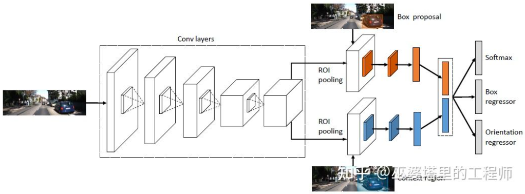
Deep3DBox [12] is one of the early and representative works in this field. A 3D object box requires 9 variables to represent, which are center, size, and orientation (3D orientation can be simplified as yaw, thus becoming 7 variables). 2D object detection in images can provide a 2D object box containing 4 known variables (2D center and 2D size), which is insufficient to solve variables with 7 or 9 degrees of freedom. Among these three sets of variables, the size and orientation are relatively closely related to visual features. For example, the 3D size of an object is highly correlated with its category (pedestrian, bicycle, car, bus, truck, etc.), and the object category can be predicted through visual features. For the 3D position of the center point, it is difficult to predict solely based on visual features due to the ambiguity generated by perspective projection. Therefore, Deep3DBox proposes to first estimate the object size and orientation using the image features within the 2D object box. Then, a 2D/3D geometric constraint is used to solve for the 3D position of the center point. This constraint is that the projection of the 3D object box on the image is tightly surrounded by the 2D object box, meaning that at least one corner of the 3D object box can be found on each edge of the 2D object box. With the previously predicted size and orientation, together with the camera’s calibration parameters, the 3D position of the center point can be solved.
!Geometric constraints between 2D and 3D object boxes (image source from reference [9])
![Geometric constraints between 2D and 3D object boxes (image source from reference [9])](https://upload.42how.com/article/image_20220114005133.png)
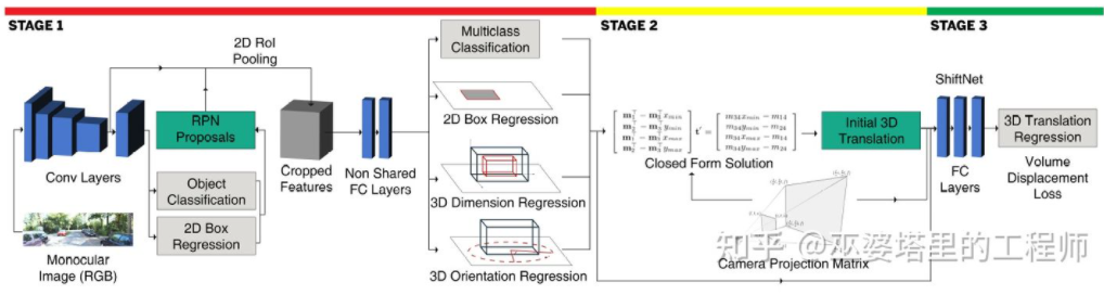
This method of using 2D/3D constraints requires extremely accurate 2D object box detection. In the framework of Deep3DBox, even small errors in the 2D object box may result in the failure of 3D object box prediction. The first two stages of Shift R-CNN [13] are very similar to Deep3DBox, which predict the 3D size and orientation through the 2D object box and visual features, and then solve for the 3D position through geometric constraints. However, Shift R-CNN adds a third stage, which combines the 2D object box, 3D object box, and camera parameters obtained in the first two stages as input, and uses a fully connected network to predict a more accurate 3D position.
 When using 2D/3D geometric constraints, the above methods obtain the 3D position of objects by solving a set of over-constrained equations as a post-processing step, which is not part of the neural network. The first and third stages of Shift R-CNN are also trained separately. MVRA [14] constructs a network for solving this over-constrained equation and designs the IoU Loss in image coordinates and the L2 Loss in BEV coordinates to measure the error in object detection and distance estimation, assisting in end-to-end training. Consequently, the quality of predicting object 3D position also provides feedback to the previous predictions of 3D size and orientation.
Directly Generating 3D Bounding Boxes
The previously introduced three methods all start from 2D images. Some transform the images into BEV views, some detect 2D keypoints and match them with 3D models, and others use geometric constraints of 2D and 3D bounding boxes. In addition, there is another type of method that starts from dense 3D object candidates, scores all candidates using 2D image features, and outputs the ones with the highest scores. This strategy is similar to the traditional sliding window method in object detection.
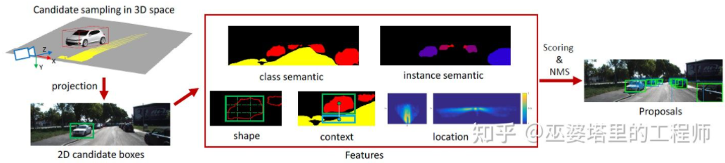
Mono3D [15] is a representative of this type of method. Firstly, dense 3D bounding boxes are generated based on prior knowledge of the object’s position (z-coordinate at ground level) and size. On the KITTI dataset, approximately 40K (vehicles) or 70K (pedestrians and bicycles) candidate boxes are generated per frame. These 3D candidate boxes are projected onto image coordinates and scored using 2D image features. These features come from semantic segmentation, instance segmentation, context, shape, and position prior information. All of these features are combined to score the candidate boxes, and higher-scoring candidates are selected as the final candidates. These candidates then undergo further CNN evaluation to obtain the final 3D bounding boxes.
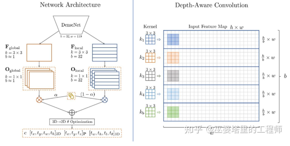
 The M3D-RPN [16] is an anchor-based method that defines both 2D and 3D anchors which represent 2D and 3D object boxes respectively. The 2D anchors are densely sampled from the image while the 3D anchors are parameterized based on prior knowledge learned from the training set data. Specifically, each 2D anchor is matched with the annotated 2D object box in the image through IoU, and the corresponding mean 3D object box is used to define the parameters of the 3D anchor. It is worth noting that M3D-RPN simultaneously employs both standard convolution operation (with spatial invariance) and Depth-Aware convolution. The latter partitions the image rows (Y-coordinates) into multiple groups, each corresponding to different scene depths, and uses different convolution kernels to process them.

Although Mono3D and M3D-RPN utilize some prior knowledge, they still rely on densely sampled object candidates or anchors, resulting in a large amount of calculation and limitations in practicality. Some subsequent methods have proposed to use the 2D detection results to further reduce the search space.
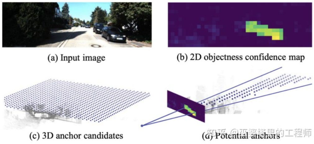
TLNet [17] densely places anchors on the 2D plane with an interval of 0.25 meters, facing 0 and 90 degrees, and a size equal to the average value of the target. The 2D detection results form multiple viewing cones in 3D space, through which a large number of background anchors can be filtered out to improve the efficiency of the algorithm. The filtered anchors are projected onto the image and the features obtained through ROI Pooling are used to further refine the parameters of 3D object boxes.
 # Translation
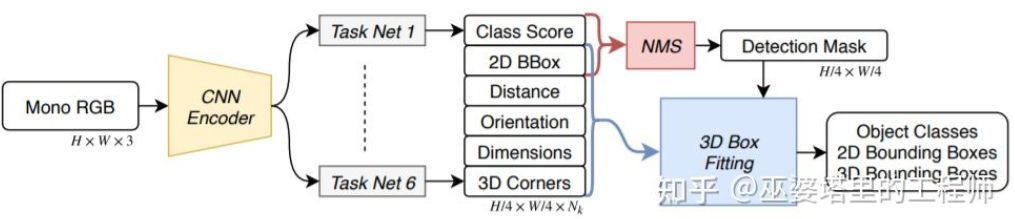
SS3D [18] utilizes a more efficient one-stage detection approach by adopting a network structure similar to CenterNet, which directly outputs multiple 2D and 3D information from the image, such as object category, 2D object box, and 3D object box. It should be noted that the 3D object box here is not a general 9D or 7D representation (which is difficult to predict directly from the image), but a 26D feature that is easier to predict from the image and contains more redundancy. This feature includes distance (1D), orientation (2D, sine and cosine), size (3D), and 16 image coordinates (8 corner points) of the 3D object box. In addition to the 4D representation of the 2D object box, there are a total of 26D features used for 3D object box prediction. All of these features are used to find a 3D object box that matches the 26D feature most accurately. A special point is that this solving process is conducted within the neural network and therefore must be differentiable, which is one of the major highlights of this article. Thanks to its simple structure and implementation, SS3D can achieve a running speed of 20 FPS.
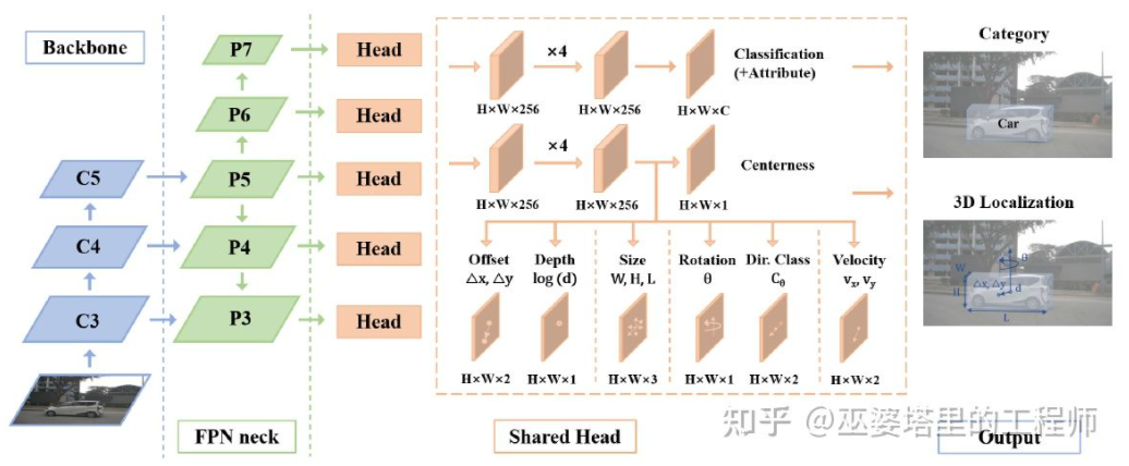
FCOS3D [19] is also a one-stage detection method, but it is more concise than SS3D. The center of the 3D object box is projected to the 2D image, and the 2.5D center (X, Y, Depth) is obtained as one of the regression targets. In addition, the other regression targets are the 3D size and orientation, where the orientation is represented by a combination of angle (0-pi) and heading.
SMOKE [20] proposes a similar idea, which directly predicts 2D and 3D information from the image through a structure similar to CenterNet. The 2D information includes the projection location of the object keypoints (center point and corner points) onto the image, and the 3D information includes the depth, size, and orientation of the center point. The 3D position of each corner point can be recovered through the 3D size and orientation, and the 3D position of the object can be reconstructed through the image position and the depth of the center point.The idea behind these several single-stage networks is to directly regress 3D information from images without complicated pre-processing (such as image inverse transformation) and post-processing (such as 3D model matching) or accurate geometric constraints (such as 3D object box corners on each edge of 2D object box). These methods only use a small amount of prior knowledge, such as the mean size of various objects in reality, and the corresponding relationship between 2D object size and depth. These prior knowledge defines the initial value of object 3D parameters, and the neural network only needs to regress the deviation from the actual value, which greatly reduces the search space and thus reduces the difficulty of network learning.
Depth estimation
The previous section introduced the representative methods of monocular 3D object detection, from early image transformation, 3D model matching, and 2D/3D geometric constraints to recent direct prediction of 3D information through images. The change in this idea is largely due to the progress of convolutional neural networks in depth estimation. Most of the single-stage 3D object detection networks introduced earlier include a depth estimation branch. Although the depth estimation here is only at the sparse object level, not the dense pixel level, it is already sufficient for object detection.
In addition to object detection, there is another important task in automated driving perception, which is semantic segmentation. The most direct way to extend semantic segmentation from 2D to 3D is to use dense depth maps, so that the semantics and depth information of each pixel are available.
Combining the above two points, monocular depth estimation plays a very important role in 3D perception tasks. From the introduction of 3D object detection methods in the previous section, it can be inferred that fully convolutional neural networks can also be used for dense depth estimation. Next, we will introduce the current development of this direction.
The input of monocular depth estimation is an image, and the output is also an image (generally the same size as the input), where each pixel value corresponds to the scene depth of the input image. This task is somewhat similar to image semantic segmentation, except that semantic segmentation outputs the semantic classification of each pixel. Of course, the input can also be a video sequence, utilizing additional information from camera or object motion to improve the accuracy of depth estimation (corresponding to video semantic segmentation).As mentioned earlier, predicting 3D information from 2D images is an ill-posed problem, so traditional methods use geometric and motion cues, combined with handcrafted features, to predict pixel depth. Similar to semantic segmentation, superpixels and conditional random fields (CRFs) are also often used to improve the accuracy of estimation. In recent years, deep neural networks have made breakthrough progress in various image perception tasks, and depth estimation is no exception. A large amount of work has shown that deep neural networks can learn superior features than handcrafted designs through training data. This section mainly introduces supervised learning-based methods. Other unsupervised learning approaches, such as utilizing binocular disparity information, dual-pixel differences from a single image, video motion information, etc., will be discussed later.
One early representative work in this direction is the method proposed by Eigen et al. [21], which is based on the fusion of global and local cues. The ambiguity of monocular depth estimation mainly comes from the global scale. For example, a real room and a toy room may look similar in the image, but the actual depth of field difference is significant. Although this is an extreme example, there are still size differences in rooms and furniture in real datasets. Therefore, this method proposes to perform multi-layer convolution and downsampling on the image to obtain descriptive features of the entire scene to predict global depth. Then, another local branch (relatively higher resolution) is used to predict the local depth of the image. Here, the global depth is used as an input to assist the prediction of local depth for the local branch.
!Global and Local Information Fusion [21]
![Global and Local Information Fusion [21]](https://upload.42how.com/article/image_20220114005326.png)
Reference [22] further proposes the use of multi-scale feature maps output by convolutional neural networks to predict depth maps at different resolutions (there are only two resolutions in [21]). These feature maps of different resolutions are fused through continuous MRF to obtain the depth map corresponding to the input image.
!Multi-Scale Information Fusion [22]
![Multi-Scale Information Fusion [22]](https://upload.42how.com/article/image_20220114005336.png)
Both of the above papers use convolutional neural networks to regress depth maps, and another approach is to transform the regression problem into a classification problem, i.e., dividing continuous depth values into discrete intervals, and each interval serving as a category. A representative work in this direction is DORN [23]. The neural network in the DORN framework is also an encoding-decoding structure, but with some differences in details, such as adopting fully connected layers for decoding and using dilated convolution for feature extraction.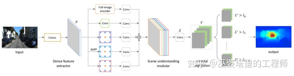
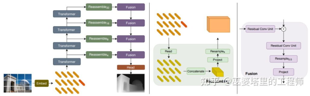
As mentioned earlier, depth estimation has similarities with semantic segmentation tasks, so the size of receptive field is also very important for depth estimation. In addition to pyramid structures and dilated convolutions mentioned above, the recently popular Transformer structure has a global receptive field, which is also very suitable for this type of task. In literature [24], it is proposed to use Transformer and multi-scale structures to simultaneously ensure the local accuracy and global consistency of predictions.
Binocular 3D Perception
Although prior knowledge and contextual information in the image can be used, the accuracy of monocular 3D perception is not entirely satisfactory. Especially when using a deep learning strategy, the accuracy of the algorithm is highly dependent on the size and quality of the dataset. For scenes not appearing in the dataset, the algorithm will have significant bias in depth estimation and object detection.
Binocular vision can solve the ambiguity caused by perspective transformation, so theoretically it can improve the accuracy of 3D perception. However, binocular vision requires high hardware and software requirements. On the hardware side, it requires two precisely aligned cameras, and the correctness of alignment needs to be maintained during the operation of the vehicle. On the software side, the algorithm needs to process data from two cameras simultaneously, and the computational complexity is high. It is even more difficult to ensure the real-time performance of the algorithm.
Overall, compared with monocular visual perception, the workload of binocular visual perception is relatively small. In the following sections, we will select several typical articles for introduction. In addition, there are some works based on multi-ocular vision, but they are more focused on the level of system application, such as Tesla’s 360 ° perception system demonstrated at AI Day. This part of content will be described in detail when introducing different perception system solutions later.
Object Detection# Translation:
3DOP [25] firstly generates depth maps from images captured by binocular cameras, and then converts the depth maps into point clouds, which are further quantized into mesh data structures for generating 3D object proposals. The generation of proposals uses intuition and prior knowledge, such as ensuring that the point cloud density in the proposal box is high enough, the height is consistent with the real object, and the height difference with the point cloud outside the box is large enough, and the overlap between the proposal box and Free Space is small enough. Through these conditions, approximately 2K 3D object proposals are sampled in 3D space. These proposals are mapped to 2D images and feature extraction is performed through ROI Pooling, used for predicting the category of the object and refining the object box. The input of the images can be either RGB images from one camera or depth maps.
Overall, this is a two-stage detection method. The first stage uses depth information (point clouds) to generate object proposals, and the second stage further refines the proposals using image information (or depth). Theoretically, LiDAR can also be used instead of the point cloud generation in the first stage, and the author has conducted experimental comparisons as well. LiDAR’s advantage lies in its accurate distance measurement, which works well for small objects, partially buried objects, and distant objects. The advantage of binocular vision is that the point cloud density is high, making it more effective in scenarios where there is little obstruction and the objects are relatively large. Of course, under the premise of not considering cost and computational complexity, the combination of the two can achieve the best results.
3DOP and Pseudo-LiDAR [3] introduced in the previous section have similar ideas. Both convert dense depth maps (from monocular, binocular or even low-line LiDAR) into point clouds, and then apply algorithms in the field of point cloud object detection.
In this process that estimates the depth map from images, generates point clouds from depth maps and then applies point cloud detection algorithms, each step is done independently and cannot be trained end-to-end. DSGN [26] proposes a single-stage algorithm that generates 3D representations in BEV views from left and right images via an intermediate representation called Plane-Sweep Volume. It also performs depth estimation and object detection simultaneously. All steps in this process can be differentiated, so end-to-end training is possible.
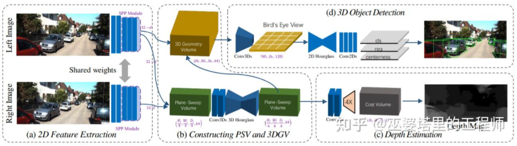 # Translated English Markdown Text with HTML tags
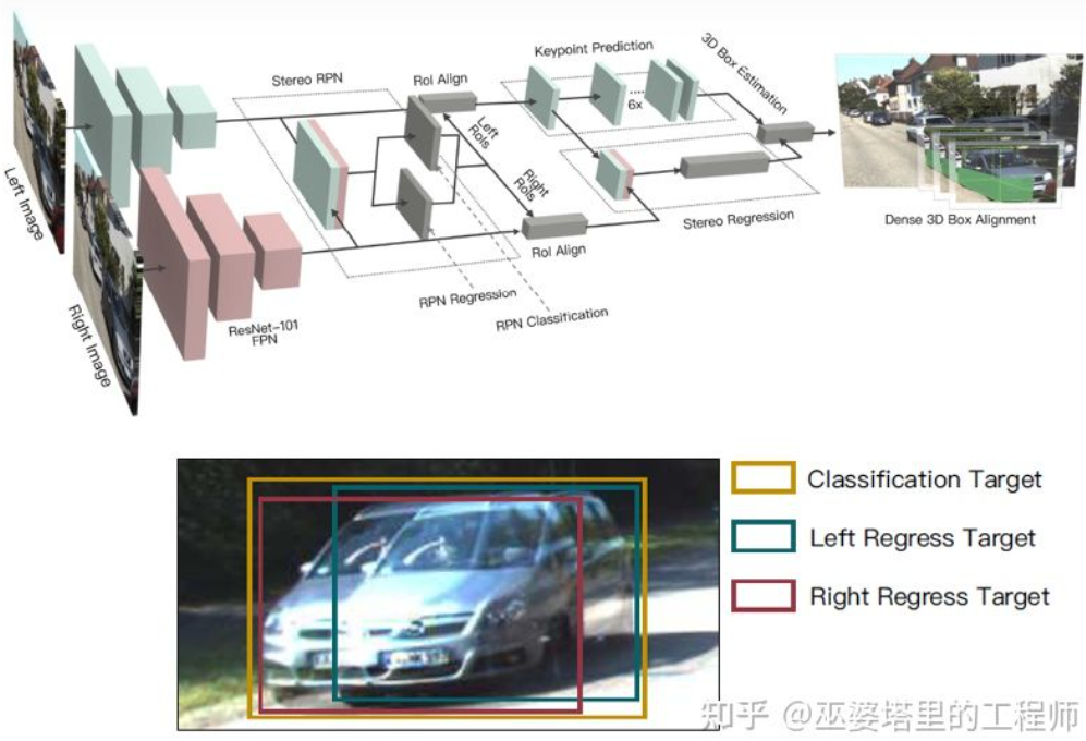
Depth map is a dense representation, which doesn’t need to obtain depth information at all locations in the scene for object learning, but only needs to estimate it at the position of interested object. Similar ideas have been mentioned before when introducing monocular algorithm. Stereo R-CNN[27] doesn’t estimate depth map, but stacks the feature maps from two cameras together under the framework of RPN to generate object candidates. The key to associating the information from left and right cameras lies in the change of annotation data. As shown in the figure below, in addition to the left and right bounding boxes, the union of the left and right bounding boxes is added. Anchors with IoU greater than 0.7 with either the left or right bounding boxes and those with IoU less than 0.3 with the union box are selected as positive and negative samples, respectively. Positive anchors will simultaneously regress the position and size of the left and right bounding boxes. In addition to object boxes, this method also uses corner points as auxiliaries. With all these information, the 3D object boxes can be recovered.
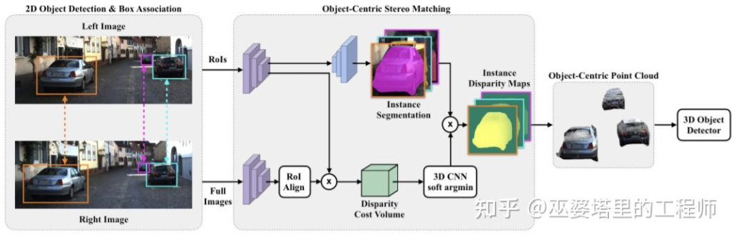
Estimating dense depth for the entire scene may even have a negative impact on object detection. For example, deep estimation deviation for object edges due to overlap with the background, and the large range of scene depth may also affect the speed of the algorithm. Therefore, similar to Stereo RCNN, document [28] also proposes to estimate depth only at the location of interested objects and generate point cloud only on the objects. These object-centric point clouds are finally used to predict the 3D information of objects.
Depth Estimation
Similar to monocular perception algorithm, depth estimation is also a key step in binocular perception. From the introduction of binocular object detection in the previous section, many algorithms use depth estimation, including scene-level depth estimation and object-level depth estimation. Next, let’s briefly review the basic principles and representative works of binocular depth estimation.
The principle of binocular depth estimation is actually very simple, which is to estimate the depth of the 3D point based on the distance d between the same 3D point on the left and right images (assuming that the two cameras maintain the same height, so only consider the horizontal distance), the focal length f of the camera, and the distance B (baseline length) between the two cameras.
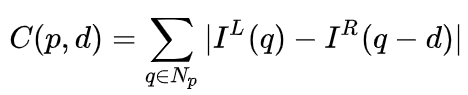
In a stereo system, f and B are fixed, so only the distance d, also known as disparity, needs to be estimated. For each pixel, the task is to find its matching point in the other image. The range of distance d is limited, so the search range for the matching point is also limited. For each possible value of d, the matching error at each pixel can be calculated to create a three-dimensional error data, known as the Cost Volume. When calculating the matching error, the local region around the pixel is generally considered, and one simple method is to sum the differences of corresponding pixel values in the local region:

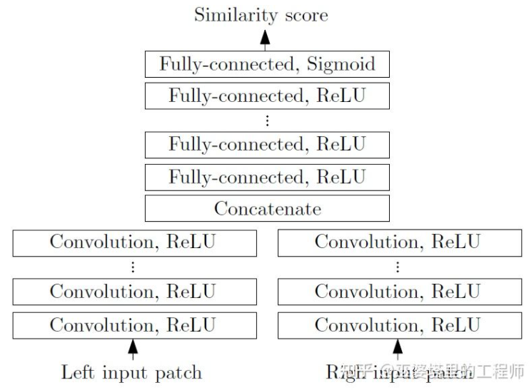
MC-CNN [29] formalizes the matching process by calculating the similarity between two image blocks and learns the features of the image blocks through neural networks. A training set can be constructed with annotated data. At each pixel, a positive sample and a negative sample are generated, each consisting of a pair of image blocks. The positive sample comes from two image blocks at the same 3D point (with the same depth), while the negative sample comes from two image blocks at different 3D points (with different depths). To maintain balance between positive and negative samples, only one negative sample is randomly selected. With positive and negative samples, the neural network can be trained to predict similarity. The core idea here is to use supervised signals to guide the neural network to learn image features suitable for the matching task.
 MC-Net has two main drawbacks: 1) the calculation of Cost Volume depends on local image blocks, which can lead to large errors in areas with few textures or repeated patterns; 2) the post-processing step relies on manual design, which takes a lot of time and is difficult to ensure optimality. GC-Net [30] has made improvements in these two aspects. First, multi-layer convolution and downsampling are performed on the left and right images to better extract semantic features. For each disparity level (in pixels), the left and right feature maps are aligned (pixel offset) and then concatenated to obtain the feature map for that disparity level. All feature maps for different disparity levels are combined to obtain a 4D Cost Volume (height, width, disparity, feature). The Cost Volume only contains information from a single image, and there is no interaction between images. Therefore, the next step is to use 3D convolution to process the Cost Volume, which can extract both the correlation information between the left and right images and the information between different disparity levels. The output of this step is a 3D Cost Volume (height, width, disparity). Finally, we need to take the Argmin along the disparity dimension to obtain the optimal disparity value, but the standard Argmin cannot be derived. GC-Net uses Soft Argmin to solve the derivation problem, so that the entire network can be trained end-to-end.
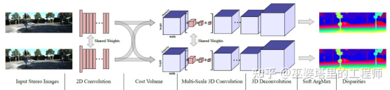
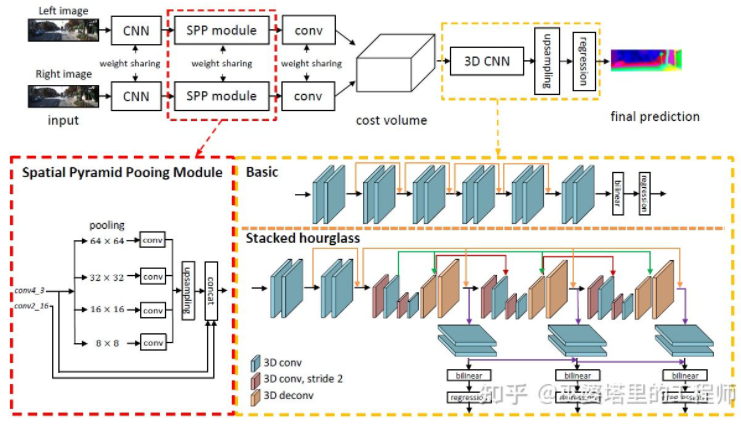
PSMNet [31] has a structure very similar to GC-Net, but it has made improvements in two aspects: 1) using pyramid structure and dilated convolution to extract multi-resolution information and expand the receptive field. Thanks to the fusion of global and local features, the estimation of Cost Volume is more accurate. 2) Using multiple stacked Hour-Glass structures to enhance 3D convolution. The utilization of global information is further strengthened. Overall, PSMNet has made improvements in the utilization of global information, making the estimation of disparity more dependent on context information at different scales rather than local information at the pixel level.
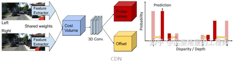
 In Cost Volume, the disparity level is discrete (in pixels), and the neural network learns the distribution of cost at these discrete points, with the extremum corresponding to the current position’s disparity value. However, the disparity (depth) value should actually be continuous, and estimating it with discrete points will introduce errors. The concept of continuous estimation was proposed in CDN [32], which estimates both the distribution of discrete points and the offset at each point. Together, the discrete points and offsets constitute continuous disparity estimation.
References
[1] Kim et al., Deep Learning based Vehicle Position and Orientation Estimation via Inverse Perspective Mapping Image, IV 2019.
[2] Roddick et al., Orthographic Feature Transform for Monocular 3D Object Detection, BMVC 2019.
[3] Wang et al., Pseudo-LiDAR from Visual Depth Estimation: Bridging the Gap in 3D Object Detection for Autonomous Driving, CVPR 2019.
[4] You et al., Pseudo-LiDAR++: Accurate Depth for 3D Object Detection in Autonomous Driving, ICLR 2020.
[5] Weng and Kitani, Monocular 3D Object Detection with Pseudo-LiDAR Point Cloud, ICCV 2019.
[6] Vianney et al., RefinedMPL: Refined Monocular PseudoLiDAR for 3D Object Detection in Autonomous Driving, 2019.- [7] Chabot et al., Deep MANTA: A Coarse-to-fine Many-Task Network for Joint 2D and 3D Vehicle Analysis from Monocular Image, CVPR 2017.
- [8] Kundu et al., 3D-RCNN: Instance-level 3D Object Reconstruction via Render-and-Compare, CVPR 2018.
- [9] Qin et al., MonoGRNet: A Geometric Reasoning Network for Monocular 3D Object Localization, AAAI 2019.
- [10] Barabanau et al., Monocular 3D Object Detection via Geometric Reasoning on Keypoints, 2019.
- [11] Bertoni et al., MonoLoco: Monocular 3D Pedestrian Localization and Uncertainty Estimation, ICCV 2019.
- [12] Mousavian et al., 3D Bounding Box Estimation Using Deep Learning and Geometry, CVPR 2016.
- [13] Naiden et al., Shift R-CNN: Deep Monocular 3D Object Detection with Closed-Form Geometric Constraints, ICIP 2019.
- [14] Choi et al., Multi-View Reprojection Architecture for Orientation Estimation, ICCV 2019.
- [15] Chen et al., Monocular 3D Object Detection for Autonomous Driving, CVPR 2016.- [16] Brazil and Liu, M3D-RPN: Monocular 3D Region Proposal Network for Object Detection, ICCV 2019.
- [17] Qin et al., Triangulation Learning Network: from Monocular to Stereo 3D Object Detection, CVPR 2019.
- [18] Jörgensen et al., Monocular 3D Object Detection and Box Fitting Trained End-to-End Using Intersection-over-Union Loss, 2019.
- [19] Wang et al., FCOS3D: Fully Convolutional One-Stage Monocular 3D Object Detection, 2021.
- [20] Liu et al., SMOKE: Single-Stage Monocular 3D Object Detection via Keypoint Estimation, CVPRW 2020.
- [21] Eigen, et al.,Depth Map Prediction from a Single Image using a Multi-Scale Deep Network, NIPS 2014.
- [22] Xu et al., Monocular Depth Estimation using Multi-Scale Continuous CRFs as Sequential Deep Networks, TPAMI 2018.
- [23] Fu et al., Deep Ordinal Regression Network for Monocular Depth Estimation, CVPR 2018.
- [24] Ranftl et al., Vision Transformers for Dense Prediction, ICCV 2021.- [25] Chen et al., 3D Object Proposals using Stereo Imagery for Accurate Object Class Detection, TPAMI 2017.
- [26] Chen et al., DSGN: Deep Stereo Geometry Network for 3D Object Detection, CVPR 2020.
- [27] Li et al., Stereo R-CNN based 3D Object Detection for Autonomous Driving, CVPR 2019.
- [28] Aon et al., Object-Centric Stereo Matching for 3D Object Detection, CVPR 2020.
- [29] Zbontar and LeCun. Stereo matching by training a convolutional neural network to compare image patches, JMLR 2016.
- [30] Kendall, et al., End-to-end learning of geometry and context for deep stereo regression, ICCV 2017.
- [31] Chang and Chen et al., Pyramid Stereo Matching Network, 2018.
- [32] Garg et al., Wasserstein Distances for Stereo Disparity Estimation, NeurIPS, 2020.
This article is a translation by ChatGPT of a Chinese report from 42HOW. If you have any questions about it, please email bd@42how.com.