Author: Haowen Sun from Pony.ai
Introduction: The pursuit of “safety first” in the development of autonomous driving technology is beyond doubt, but comfort may be overlooked in the process.
Therefore, today I want to share with you how autonomous driving development can achieve a balance between safety and passenger comfort through optimized algorithms in the planning and control modules.
Definition of Safety and Comfort
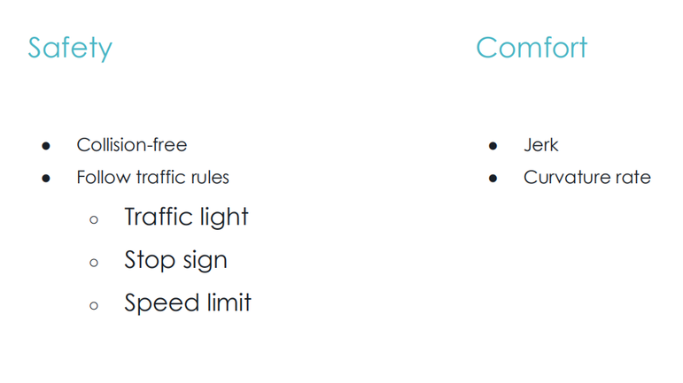
The definition of safety is relatively easy to understand, generally including not colliding and obeying traffic rules (traffic lights, parking signs, speed limits).
Comfort is influenced by the following two indicators:
-
Jerk, which is the rate of change of acceleration. The smaller the rate of change of acceleration, the more comfortable the passenger feels.
-
Curvature rate, which is the rate of change of curvature. The smaller the rate of change of curvature, the more comfortable the passenger feels.
Based on the definitions of the two, “safety and comfort are not mutually exclusive” implication means controlling the rate of acceleration and curvature of the traveling route while complying with traffic regulations and not colliding.
Definition of Planning and Control
Planning and Control are the bottom-most parts of the autonomous driving system, determining how the car drives on the road.
Generally, the input information required for planning includes map information, start and end points, obstacle predictions, traffic signs, and perception information, such as the position, size, speed, and direction of objects in the environment.
With these inputs, the planning module can output a trajectory of a certain period of time, which is the function (Xt~Yt) of the position the vehicle reaches at a certain time.
The output trajectory of the planning is one of the two inputs of the control module. The other input is the vehicle’s self-state, including the vehicle’s position, heading, speed, acceleration, angular velocity, and so on.
The control module will output the following two types of information:
- Brake/throttle pedal
- Steering angle
Simply put, the purpose of control is to enable the autonomous vehicle to accurately implement the driving instructions given by the planning module.
The above is a simple definition of planning and control. Of course, I also leave a question for you to think about (the gray area in the figure above): is it necessary for the planning module to know the vehicle’s real-time location information?## How to ensure safety and comfort in planning?
Safety
As mentioned before, the goal of planning is to output a trajectory (a function of time to position): X (t) = (x (t), y (t)) T. This driving path needs to ensure both safety and comfort.
In fact, planning is an optimization problem. For an optimization problem, we need to design constraints to ensure safe driving.
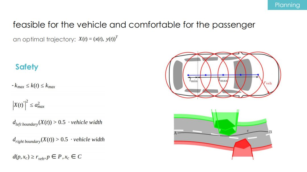
The above figure lists some of the most basic constraints.
Firstly, the planning module cannot ignore the physical characteristics of the vehicle, such as the maximum angle of the steering wheel, which corresponds to the maximum and minimum values of curvature, etc.
Secondly, the limits of braking and acceleration of the vehicle should be clear, which corresponds to the limit of acceleration.
Thirdly, when the autonomous driving vehicle is driving on the road, in order to avoid crossing the lane line, the distance between the vehicle and the left and right boundaries (lane lines) also needs to be included in the planning.
Fourthly, the autonomous driving vehicle certainly does not want any collisions. We can cover the vehicle’s body by taking a series of circles with equal radii on the vehicle axis, and use several convex polygons to represent the objects around the vehicle’s body. Therefore, when the distance from all circle centers on the vehicle axis to the convex polygon is greater than the radius, the autonomous driving vehicle will not collide with the convex polygon (obstacle).
Comfort
After introducing safety, this section will explain how the planning module achieves driving comfort. As mentioned before, the higher the comfort, the smaller the rate of change of acceleration and curvature. The corresponding cost function can be set as follows: acceleration + rate of change of acceleration + curvature + rate of change of curvature.
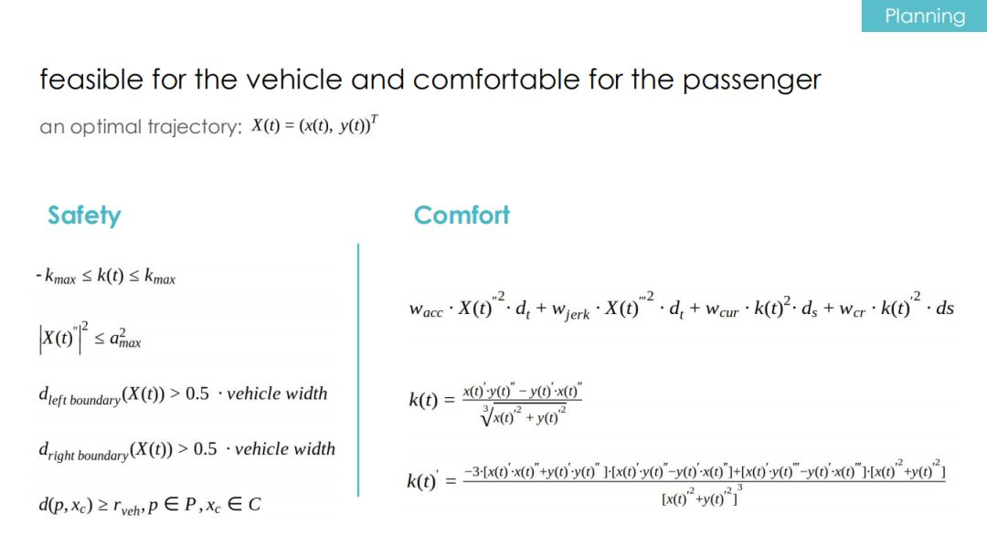
Although the entire model design is relatively simple, the solution for constraints and cost functions (as shown in the above figure) is quite complicated. Especially, in real-time, solving for k(t) and k'(t) takes a long time and is challenging. At this point, we can think of the problem differently and transform it.
As mentioned before, the planning problem is actually to solve a function of time to position. L4 autonomous driving vehicles generally run on structured roads, which also means that the planning module has map information, and the problem can be transformed by converting the (x, y) coordinate system to the (l, s) coordinate system shown in the figure below.# Translated English Markdown text with HTML tags
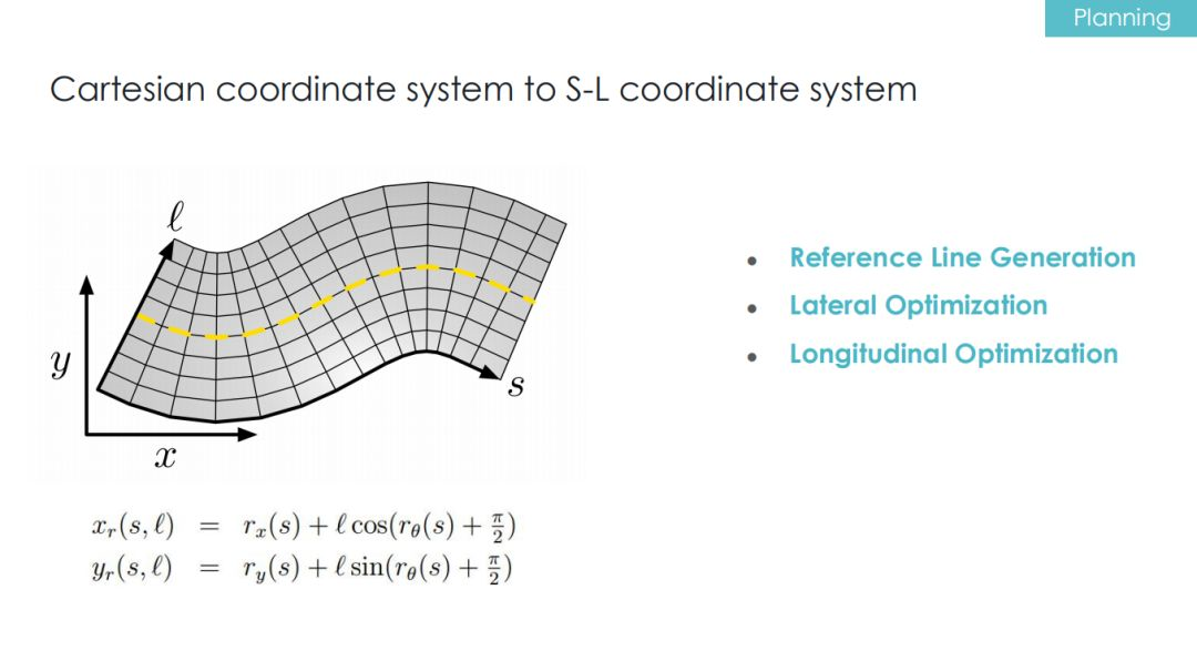
The longitudinal direction of the car is denoted by s along the reference line, whereas l is the direction perpendicular to the reference line. Therefore, the problem is reduced to finding solutions for s(t) and l(s). We want to determine the position on s where the autonomous vehicle should be at time t, as well as how far the car deviates from s to the left or right at that position.
Eventually, a complex problem is transformed into three sub-optimisation problems: one for lateral control, one for longitudinal control, and one for the reference line (where s direction is longitudinal planning, and l direction is horizontal planning).
Now, I will explain each sub-problem in detail.
Sub-Problem 1: Lateral Control
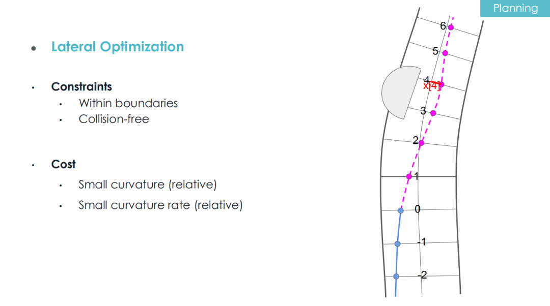
On the right side of the above figure, a road is displayed, with the reference line in the middle. The point labeled “0” is where the car is currently located, while “-1,” “-2” represents previous coordinates, and the following points, labeled “1,” “2,” “3,” “4,” etc., are the output of the planning module, showing the car’s future positions.
The boundaries or lane markings are on both sides of the road, and the half-circle in the figure represents an obstacle on the road surface. Lateral planning aims to solve the value of l for each point, which indicates the deviation from the centerline.
For the lateral control problem, we consider safety and comfort from two aspects.
For safety, it depends on the constraints of lateral optimization. Generally, l should not be too small or too large, meaning the car should not hug the left or right boundary, nor should it hit the obstacles on both sides.
For comfort, we design a cost function to minimize the curvature of the path and its rate of change. If the reference line is a perfect curve, the curvature can be represented by relative curvature ratio.
As for an optimization problem, the cost function becomes a standard quadratic function, and all constraints are linear.
Thus, it becomes a standard QP (quadratic programming) problem with box constraints, enabling us to obtain the optimal solution quickly.
Sub-Problem 2: Longitudinal Control
Longitudinal planning solves the function of t to s.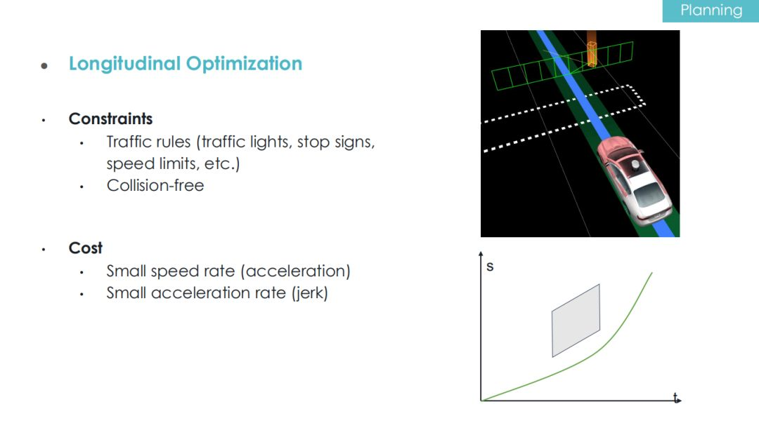
For longitudinal planning, safety requires us to ensure that the vehicle does not collide in the front or rear direction. Take the example on the right side of the figure. At this time, if a pedestrian is crossing the road, the planning module will convert the pedestrian’s behavior into (t, s) coordinates, which are displayed as a parallelogram on the coordinate graph (above).
At this point, facing the pedestrian, if the self-driving car chooses to give way, the curve solved by the longitudinal planning should be below the parallelogram; if it chooses to exceed the pedestrian, then this curve should bypass it from the top.
In longitudinal planning, comfort is reflected in the smaller the acceleration, the better, and the smaller the derivative of the acceleration, the better. It can be seen that the constraints and cost functions involved in longitudinal and lateral planning are very similar.
Sub-problem III: Centerline generation
Similarly, the generation of the centerline is also an optimization problem, so it will naturally involve constraints and cost functions.
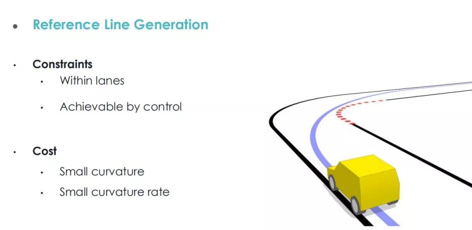
The constraints set for the centerline generation are that it cannot squeeze the boundary (lane line) and must comply with the curvature limits. For the cost function, the goal to be achieved is that the smaller the curvature of the centerline, the better, and the smaller the rate of curvature change, the better. In this way, the centerline problem is also a problem of solving the functions k(t) and k(t)’.
It seems that the problem has come back again. Do we still need to solve very complex equations for comfort?
Not really. Since the centerline can be generated offline, it does not need to be calculated online, and these problems can be parallelly calculated on the server.
Here, I would like to add a thought-provoking question. As mentioned earlier, the precondition for generating the centerline is to have information about the road, that is, the boundaries (lane lines) on both sides of the road. However, when the self-driving car is in an intersection and there are no lane lines on the road, how should the reference line be processed in this environment? Welcome to leave a comment for discussion.
How to achieve safety and comfort in control
After all, automatic driving controls a car, not just a point. So before introducing the automatic driving control module in detail, I would like to introduce a model first.
Bicycle Model
There are many models for control, and they are very complex, considering many factors of the vehicle, including the engine, gearbox, tires, suspension, and so on. To tell this problem well, I will introduce the simplest model, the Bicycle Model.
Assuming the width of an autonomous vehicle is zero, it can be imagined as two front wheels and two rear wheels leaning against each other (as shown in the figure above).
This assumption means that the steering angle and speed of the front wheels are the same. Of course, in reality, the steering angle and speed of the four wheels of a vehicle are different. Therefore, this model is only making the simplest assumption. Based on this assumption, when we know that the steering angle of the front wheels has changed by δ, we can also calculate the turning radius of the rear axle through geometric relationships.
The previous assumption of the car being a “bicycle” implies that the lateral velocity of the rear wheels is zero. Therefore, the rear wheels always travel towards the direction of the front wheels. Drawing a tangent line on the red line in the figure below shows that it does not intersect with the blue line, so it is not the rear wheel. A tangent line drawn on the blue line intersects with the red line, so the blue line is the trajectory of the rear wheel.
Which direction is the car heading? We continue to draw a tangent line on the blue line, which still has two intersection points with the red line. In fact, the distance between the intersection point and the tangent point is the wheelbase of the car. Since the wheelbase is fixed, the traveling car is shown by the black line in the figure. The answer to this question is: the red line represents the front wheels, the blue line represents the rear wheels, and it is heading to the right.
In summary, for vehicles with only two axles and steering through the front wheels, the Bicycle model can generally be used to convert them. However, on real roads, not only cars but also trucks are often driven. Trucks can be divided into two parts, the cab and the trailer.
For the control of the truck, if we still assume the Bicycle model (as shown above), A1 is the cab, A2 is the trailer, F1 is the front axle of the cab, and R2 is considered the rear axle of the trailer. In this model, we assume that the front axle of the trailer and the rear axle of the cab are the same point R1=F2, the wheelbase of the cab is L1, and the wheelbase of the trailer is L2. When we know that the front axle of the cab has turned by ϕ degrees, the control module can obtain the turning radius of the rear axle of the cab.
So, what kind of curve will the trajectory of the trailer’s rear axle show? This question is also welcome for everyone to discuss. After all, there is not only one type of vehicle on the road in real life, and autonomous driving practitioners can think about the motion behavior of various types of vehicles.Lateral Control
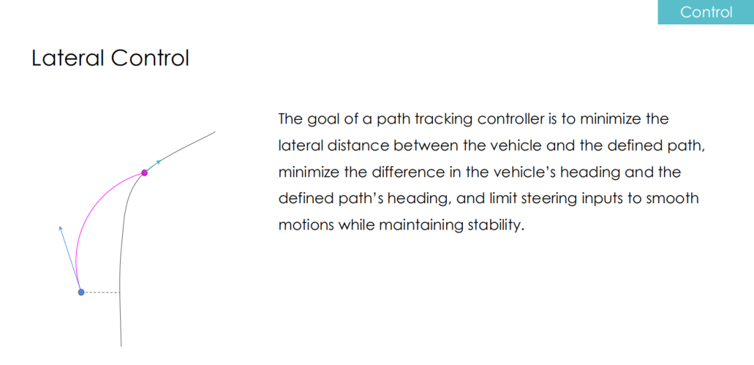
The purple curve in the above figure is the target trajectory output by the planning module. The blue dot represents the current position of the autonomous vehicle, and the blue arrow shows the current driving direction of the vehicle.
As we can see, there exists a lateral deviation between the actual trajectory of the autonomous vehicle and the planned trajectory. Therefore, the goal of lateral control is to minimize the lateral deviation between the actual trajectory and the desired trajectory as well as the heading error between the vehicle’s heading at a certain moment and the desired heading at the corresponding point on the planned trajectory.
Preview algorithm is commonly used in lateral planning. The goal of lateral control is to minimize the lateral deviation and heading error from the actual trajectory to the target trajectory at the preview point. The curvature mentioned earlier is the control variable, making lateral control an optimization problem.
Longitudinal Control
Similarly, for longitudinal control, we can also choose a preview point. The desired goal is to minimize the speed (v) error and displacement (s) error between the autonomous vehicle and the planned trajectory. Thus, longitudinal control can also be transformed into an optimization problem.
In summary, both planning and control can be transformed into optimization problems.
For exploration of comfort and safety of autonomous driving planning, the focus is on designing constraints and cost functions in optimization problems.
The control module is concerned with preview point selection, and its ultimate goal is for the autonomous vehicle to more accurately follow the planned trajectory. The closer the preview distance, the more accurate the control will be. Conversely, a farther preview distance will result in a smoother control, which may feel more comfortable, but the error can be greater.
In the end, we can sit in a safe and comfortable autonomous vehicle. This is the end of today’s sharing. Thank you all.
This article is a translation by ChatGPT of a Chinese report from 42HOW. If you have any questions about it, please email bd@42how.com.