Automated driving software framework and basic components that support Level 3 or higher functionality.

Author: Xiaomeng

Welcome to follow the series of articles “Software Architecture and Implementation of Intelligent Driving Domain Controller“. In the previous article, we shared an overview of the software architecture of the intelligent driving domain controller. This article focuses on the part related to intelligent driving in the overall software architecture described in the overview diagram, namely, the “Intelligent Driving Software Framework and Basic Components”. It provides an in-depth description of the two core frameworks in this part, namely, the “Environmental Model Framework” and the “Implementation Framework of EPX-SA Model”.

Context of Algorithm Execution

Now let’s discuss the architecture of the L.FW layer. As mentioned earlier, the semantics of “intelligent driving” are introduced from this layer onward. This semantics should be reflected in both the real-time and performance domains of the D-axis, and should also be able to support the characteristics required by various aspects of the A-axis.

As mentioned in Chapter 1, the core of autonomous driving is various types of “algorithms”. What the L.FW layer needs to provide is the carrier for running these algorithms. So, how can we make the running of algorithms that the carrier supports happen? In the following diagram, we analyze the context of algorithm execution from the three dimensions of time (T), resources (R), and data flow (F).

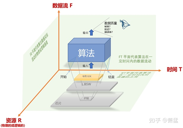
Resource Dimension

The running of any algorithm ultimately needs to be implemented on physical devices. This is particularly prominent in algorithms related to autonomous driving. The physical device on which the algorithm runs is constrained by the following factors:

• Performance and real-time requirements of the algorithm

• Limitations of the physical device itself or its SDK.“`markdown
  Some algorithms must run in real-time domains, such as radar processing algorithms. It needs to control the transmission of electromagnetic waves and receive echoes to perform analysis based on the time difference between the transmission and reception. The algorithm requires high precision in time scheduling, so it is generally run on an RTOS of MCU. If the main CPU of the MCU is not powerful enough, a DSP chip will be added to accelerate it.

The location where visual algorithms using deep learning run is related to hardware physical devices and their SDK. In most cases, their dedicated hardware modules (IP cores within chips) can only be accessed on OS such as Linux/QNX. The SDK that the algorithms require depends on the software environment on Linux/QNX since it can only run in the performance domain.

Generally, advanced SoC chips provide various resources for algorithm acceleration, including ISP modules for image signal processing, DSP modules for digital signal processing, AI modules for executing deep learning inference algorithms, GPU for supporting graphics rendering, and so on. Chip manufacturers also provide corresponding dedicated SDK. These dedicated SDKs are platform-dependent and are not part of the “L.FW autonomous driving software framework.”

The “L.FW autonomous driving software framework” needs to allocate and manage the hardware computing resources required by the algorithm. This can be divided into “hardware platform-independent” and “hardware platform-dependent” parts.

If L.FW only uses services or API interfaces provided by the lower-level L.BSW layer, it is basically “hardware platform-independent” because the L.BSW layer has shielded some platform-related low-level details.

If a hardware platform provides hardware modules that can accelerate certain algorithms, and two algorithms need to use it, then management needs to be done at the L.FW layer. Alternatively, L.FW develops corresponding abstract interfaces to shield hardware-relatedness.

Whether it is platform-dependent or platform-independent, when multiple algorithms compete for the same resource, L.FW needs to make arbitrage.

Time Dimension

As mentioned earlier, multiple algorithms may compete for the same resource. The most basic is to arrange the algorithms reasonably to avoid conflicts in time. Each algorithm should have its reasonable start and end time. However, this is precisely the most difficult part. Most intelligent driving prototype systems usually let all algorithms run together. This is possible for simple single scenes. In ECUs with single functions of L2 and below, because there are not many involved algorithms, determining the enablement or stopping of algorithms based on the state machine of single function can still be achieved.

When it comes to Level 3 and above, different algorithms required for different scenes have significant differences. Therefore, algorithm execution time management is very important. More precisely, the “L.FW autonomous driving software framework” should manage the life cycle of algorithms.
“`### Data Flow Dimension

In autonomous driving, various algorithms are not isolated and there is interaction between them in terms of data. The output of one algorithm is the input of one or more other algorithms. Multiple algorithms are cascaded to form a data stream pipeline.

However, it needs to be analyzed based on the actual situation whether all algorithms are assembled in the form of data streams. Generally speaking, perception-type algorithms are prone to show a multi-level cascaded data pipeline form. But for other algorithms, it is still debatable whether the data stream is the most appropriate mode. For example, the same “planning (P) + execution (X)” algorithm of EPX-SA fractal recursion hierarchy will form a feedback loop, and P will monitor the execution results of X and replan accordingly. Scheduling algorithms (S) need to identify scenarios and adjust the algorithm pipeline, which is more like a control mechanism outside the algorithm pipeline.

In any case, at this level, the “autopilot software framework (L.FW)” must manage the assembly and uninstallation of algorithms in the data processing flow and supervise the input and output data quality of each algorithm.

Algorithm assembly can be static or dynamic. Static assembly is described in the configuration file and needs to be restarted to take effect after modification. In the car, OTA updates are needed for configuration. Dynamic assembly dynamically determines the installation and uninstallation of algorithm modules according to the running state, and even migrates on different hardware resources dynamically.

The advantage of static assembly is strong testability, which can guarantee system reliability through complete coverage testing. The advantage of dynamic assembly is strong flexibility. Generally, automotive software tends to be statically configured for reliability. The algorithm modules of autonomous driving must be dynamically enabled or stopped, but dynamic and static are also relative. Perhaps the dynamic switching function we need can be supported by some static configuration. Specific implementation methods need to be found in the design and development, and we also need to see what available capabilities L.BSW provides at this level.

Meaning of the Three Planes

In the above figure, F, T, and R axes form a plane between any two axes.

• The FT plane represents the data flow of algorithms within a certain period of time.

• The FR plane represents the physical or logical channel of actual data flow of algorithms.

• The RT plane represents the resource usage of algorithms during a certain period of time.

This explains from another perspective what L.FW needs to do.

To summarize the above, we must be clear: The “autopilot software framework (L.FW)” does not implement specific algorithms, but it prepares the context for algorithms, that is, the resources, time, and data required for algorithm execution. It is the container for algorithm execution. Also, do not forget that L.FW includes real-time and performance domains, and there should be equivalent implementation in both domains, as well as appropriate communication mechanisms. Of course, the specific implementation architectures of the two domains are different, but what they do is within the scope mentioned above. However, the real-time domain can be greatly simplified in terms of architecture.

The Goal of Perception Algorithm Is to Build Environmental ModelsThe concept of environment model has been mentioned earlier. The environment model is an important product of the L.FW layer and will be further elaborated here.

When designing a prototype system for a single scene, we can focus only on perception, and the results of perception are used for subsequent planning, which is basically a linear model. This linear model can support the implementation of most level 2 autonomous driving functions. When each level 2 function is implemented separately, the number of sensors involved is relatively small, and the software module that needs perception data is relatively simple.

In section 2.3, the “Driving Assistance Domain Controller” can already receive various types of perception data. When these data are centrally expressed and processed, the embryonic form of the environment model has already emerged.

Exploration of the environment model

The following figure is a UML class diagram representation of the target recognition result information of Mobileye EyeQ4. The content is organized according to the DBC file of EyeQ4 output information by reverse analysis.

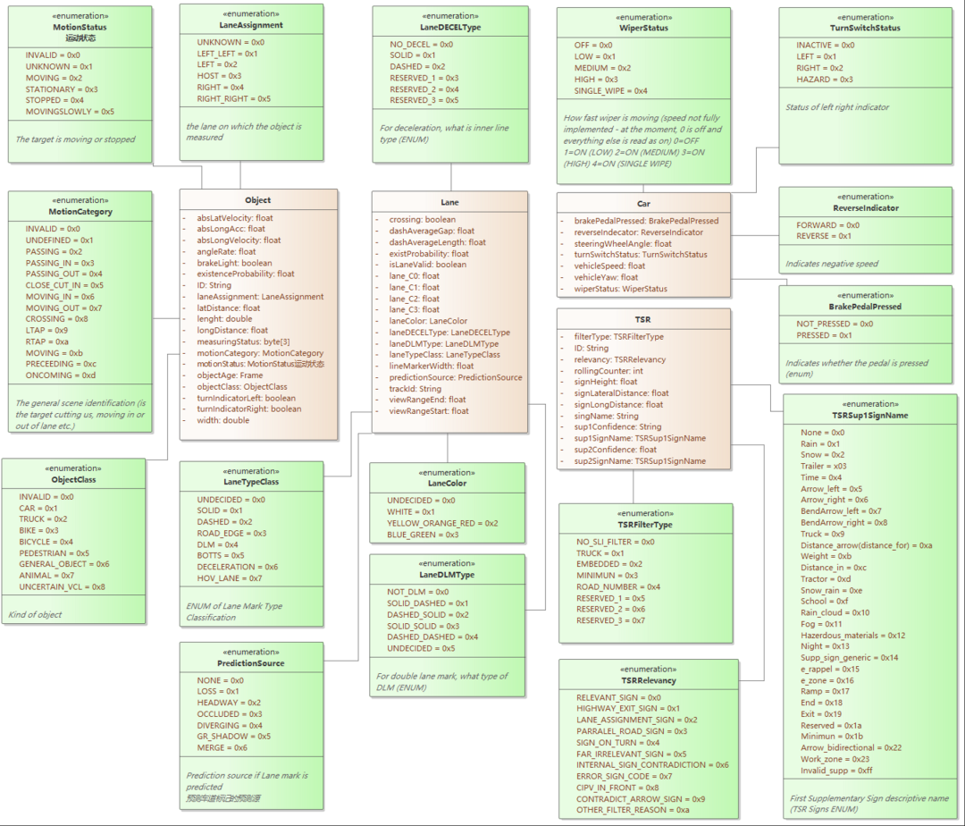
EyeQ4 belongs to Smart Sensor, which integrates visual algorithms and execution algorithms. The algorithm acceleration uses Mobile’s own dedicated chips. EyeQ4 outputs the results of visual algorithms through the Can bus. From the above figure, it can be seen that the information output by EyeQ4 mainly includes three categories:

1. Object represents all targets, ObjectClass is for target classification, including cars, trucks, bicycles, pedestrians, animals, etc. MotionStatus indicates the state of the target, whether it is stationary, moving, etc., without more specific information such as speed and direction of movement.

2. Lane represents lane lines. Lane lines can be further classified by type (solid line, dashed line, double line, etc.) and color.

3. TSR is traffic sign recognition, with detailed information including the type and semantics of the signs.

Here, LaneAssigment has a special meaning, which indicates which lane the object is in. The two types of information are combined.

EyeQ4 also needs input information. It needs current vehicle state information to better obtain and use the three types of information mentioned above. For example, to indicate which target is the vehicle in front.

EyeQ4 is a commercial product, and the above figure shows its clear external perception data interface protocol. There may be more detailed data formats inside, such as multi-level algorithm cascading, and the data interface between each level has not been disclosed. The publicly available interface data already describes part of the environment.

The “Automatic Driving Function Software Interface Standard” jointly released by Huawei and China Intelligence Connected Car defines the data interfaces for four service aspects: location, environment, prediction, and decision planning. The term in parentheses is the language used in the standard. The standard interface is defined in protobuf format. The UML class diagram was reverse analyzed and organized from the protobuf format, as shown in Figure 4.

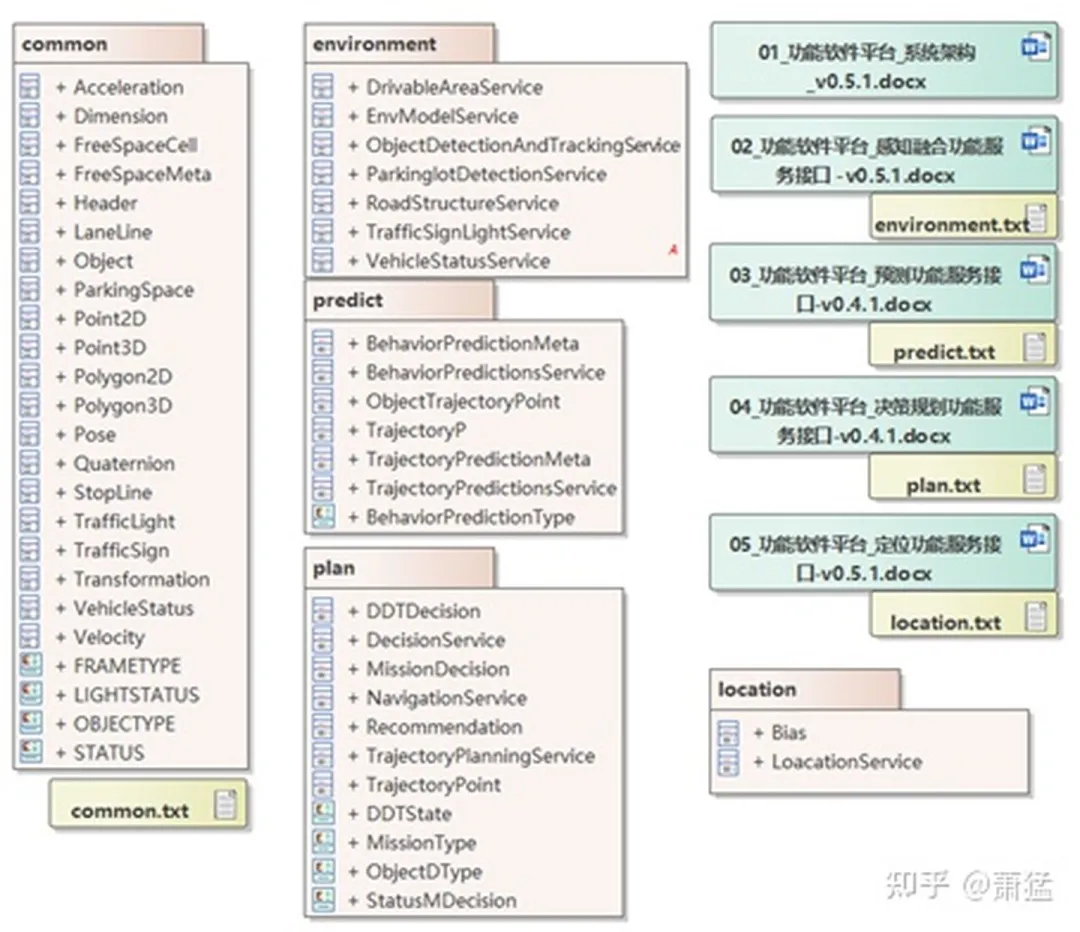
The information output by EyeQ4 is included in the “Common” part of the “Automatic Driving Function Software Interface Standard.” “Common” also includes basic data formats starting from 2D points and 3D points, parking spaces, drivable areas, and other related environmental information. For detailed information, refer to the figure below.

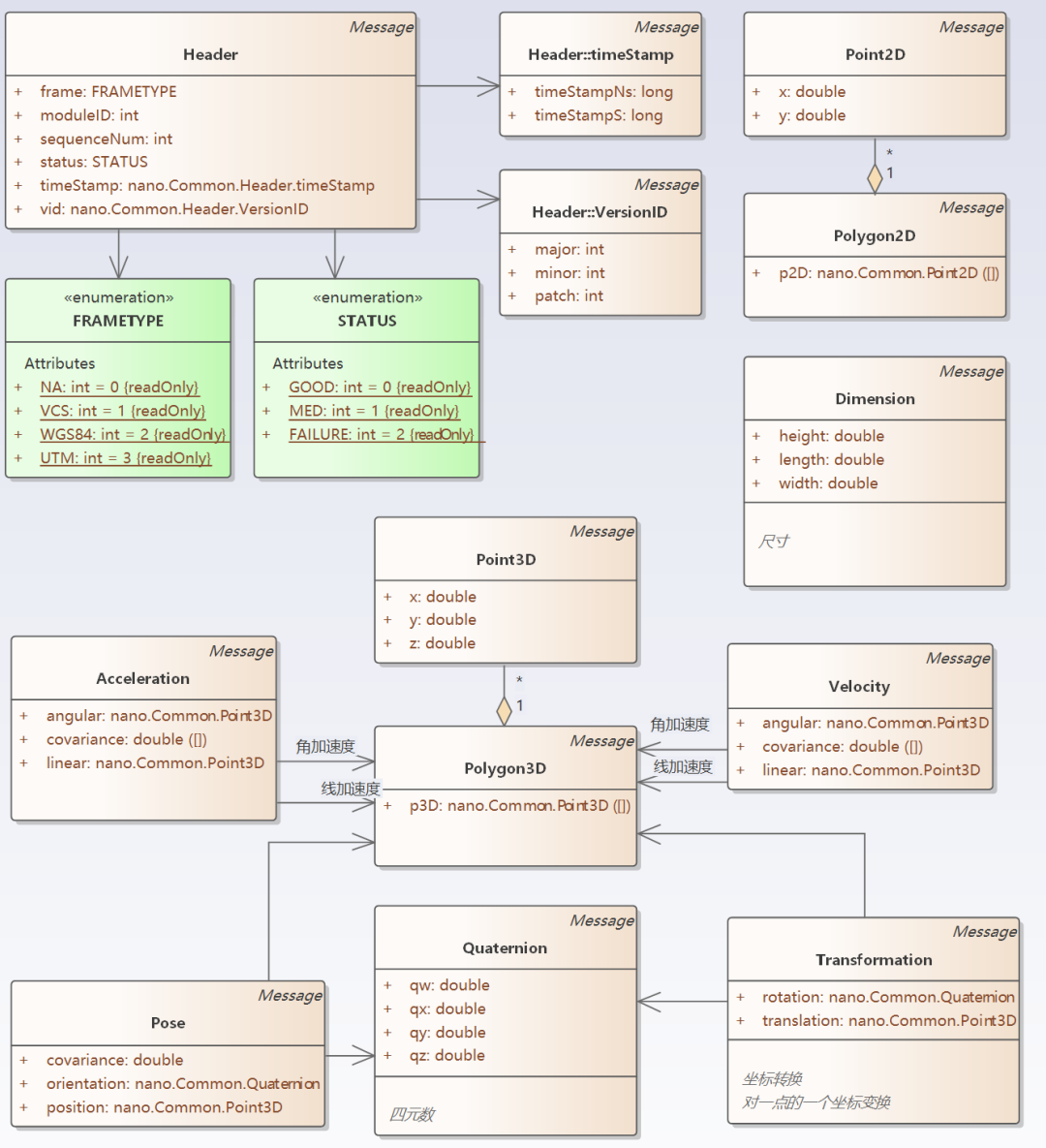
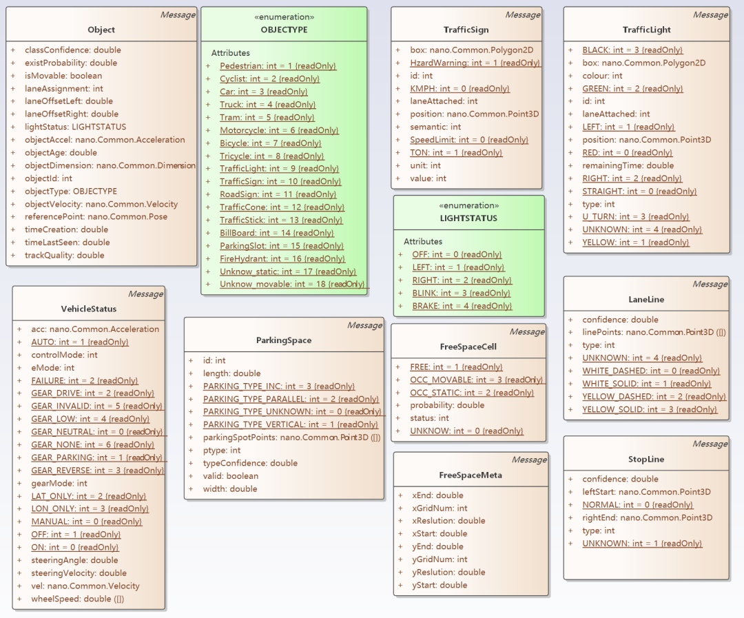
In addition, the above interface standard also includes the content of prediction and positioning. Positioning refers to a part of the vehicle information, including position, speed, posture, and the status of devices inside the vehicle such as the accelerator pedal and brake. In a narrow sense, “environment” does not include vehicle information, but only includes the environment outside the vehicle. The terms “environment” or “environmental model” mentioned in this article both include vehicle information.

The above interface standard also includes the “prediction” section, which includes behavior prediction and trajectory prediction. Behavior prediction refers to the possible behavior semantics of the “target” detected in the future, such as start, deceleration, acceleration, left turn, etc. Trajectory prediction estimates the trajectory that the “target” may travel (or walk) within a certain period of time. The above interface standard does not include these two predictions as parts of the environment.We believe that the environment not only has spatial properties, but also temporal properties. “Prediction” is the possible outcome of the environment model in the temporal dimension, and there should also be a part of the environment model that represents the “history” in the temporal dimension. In other words, “historical trajectory” and “historical behavior” are also part of the environment model. In fact, in the EQ4 environmental data, there is a field “ObjectAge” for Object, which represents how many frames the target has appeared. This already has some temporal properties. There is a type of tracking algorithm in perceptual algorithms that also belongs to temporal semantics. The concept of the environment model in this article includes the “prediction” and “history” in the temporal dimension.

Multi-level Semantics of Environment Model

Two types of hierarchical relationships

There are two types of hierarchical relationships in the environment model. One is the hierarchical relationship of the fractal recursive EPX-SA model, which reflects the granularity of the scene. Suppose there are three granularities:

• Granularity 1: We are concerned with a city-wide scene and are interested in the congestion of the road network. This information can be obtained through the vehicle network cloud for planning the driving path from point A to point B in the city. We are not interested in what cars are nearby.

• Granularity 2: We are concerned with a street level scene (within 500 meters) and are interested in the congestion of several lanes ahead and the status of traffic lights at the next two intersections. This information can be provided by the Road Side Unit (RSU) of the vehicle-infrastructure cooperative system. We still don’t need to be concerned with nearby cars at this level of granularity.

• Granularity 3: When we need to change lanes to avoid congestion based on the information from Granularity 2, we need to pay attention to the information about the surrounding vehicles and lane conditions. This information can be obtained through the sensors of our vehicle or from the RSU.

The other type is the different semantic levels from low (shallow) to high (deep) at Granularity 3. Here, “semantic” refers to structurally meaningful information with specific field significance. For example, a photo is just a meaningless set of pixels without semantic information. Recognizing “this is a person, this is a car, and that is a road” is semantic information, while judging “the person is in the car” is a deeper semantic information.

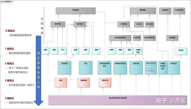
Semantic Levels

We divided semantic levels into five levels from 0 to 4, from low to high.

Level 0 is the raw physical signal without semantics, such as a set of raw pixels from a camera, a point cloud from a LiDAR, and a waveform received by a radar.

Level 1 is attribute features calculated based on the raw physical signal, biased towards physical properties (with measurement units or dimensions), such as speed, position, color, etc. It does not have semantic information related to vehicle driving.

Level 2 starts to have semantic information related to vehicle driving, such as speed limit, left turn lane, parking space, etc. Generally, it does not have physical dimensions. Geometrically feasible driving areas.## 3rd level semantics

3rd-level semantics is further processing based on 2nd-level semantics, with the following possibilities:

• Combination of two 2nd-level semantics, such as a vehicle on a certain lane.
• Simultaneous presence of both time and space dimensions, such as historical trajectory and trajectory prediction.
• Recognition and judgment of intention, such as current behavior and behavior prediction.

4th level semantics combines multiple 2nd- and 3rd-level semantics, such as the drivable area obtained by adding traffic regulations, the behavior of other targets, and trajectory prediction. At this level, the analysis is closest to planning.

As shown in the figure below, examples of semantic levels are listed. However, the focus of this section is on the analysis method of environment modeling based on semantic levels. The specific level division criteria and the level to which each semantic belongs need further research and analysis.

Why define semantic levels:

1. Semantic levels are the natural logic of perception algorithms. Defining semantic levels can clearly define the boundaries of different types of algorithm and enable each segment to focus more clearly on solving problems in its own field.

2. Facilitating collaborative work and mutual backup of multi-channel perception sources. Autonomous driving below Level 2 uses fewer sensors with low overlap. From Level 3+, more sensors are gradually deployed, and there may be functionally overlapping parts in the various sensors. At the same time, V2X technology allows us to directly receive perception data from cloud or roadside units, and this data that has been processed by cloud or roadside units directly becomes 2nd- or level semantics. Clear semantic grading is helpful for defining interface forms between different semantic levels, and different sources of semantics can be directly injected into corresponding locations in the environment modeling.

3. Low-level environmental model semantics can be used to compute multiple high-level semantics, and clear semantic grading can reuse the technology of low-level semantics and avoid duplicate calculation of high-level semantics.

4. High-level environment semantics allow for simpler and more reasonable planning algorithms. Currently, most perception algorithms achieve 1st-level semantics and some 2nd-level semantics. Higher-level semantics are frequently implemented in planning algorithms. In the EPX-SA model, each fractal recursive level of EPX may be replaced by a scheduling algorithm. Each P (planning) component needs to perform high-level semantic calculations, which will increase the complexity of the P component. High-level semantics are directly provided by specialized algorithms, and each P component uses them as needed. This makes the division of labor between perception and planning clearer, and each algorithm can focus more on its own field.

Ideal Model and Real Model

The environment model “ideal model and real model” is another dimension orthogonal to “semantic levels”.The ideal environment model assumes that all semantic data obtained from the environment are fully accurate, without delay, and cover all aspects. However, this is not always the case. The actual environment model differs from the ideal in several ways:

1. The coverage is smaller than the ideal model.

As mentioned earlier, each sensor can be seen as a filter for the environment model in terms of “angles, distances, and spectral intervals”. As shown below, a sensor combination is the union of multiple filters. However, no matter how many sensors there are, their union is still only a subset of the entire ideal environment model.

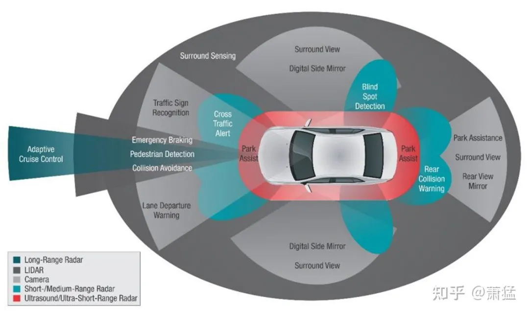
Figure 18: Sensor as a filter of the ideal environment model

2. There is delay in the data.

All sensors have a delay, and the delay accumulates gradually during multi-level transmission and calculation. A 1080p image requires about 7 milliseconds of transmission time through the fastest current transmission line GMSL2 (~6Gbps), then it goes through multiple perception algorithms, planning algorithms, and control output, which takes at least 30-50 milliseconds. A vehicle driving at 60 km/h has already traveled 0.5 to 0.8 meters.

For Level 2 and below automated driving function development, the cable and the required performance and delay of each algorithm are generally defined in the system design stage to control the total delay. The algorithm with the highest performance overhead will have exclusive access to the relevant computing acceleration resources, and efforts will be made to optimize it to meet the design requirements during development. It is equivalent to statically requiring a maximum delay range in the entire system, and each processing level guarantees that it meets its own static requirements. There is no delay-related information in the overall semantic of the environment.

For Level 3~Level 4 automated driving implementation, the granularity of various scenes will be switched according to the situation, and various algorithms will use computing resources in turn, with some algorithms competing for computing resources. Therefore, the delay of data processing will be dynamic. It is necessary to embed the delay-related information in the environment model as part of the actual model.

3. The accuracy of the data has a confidence interval, which varies with environmental factors such as day and night, and weather.

The accuracy of any algorithm’s results is a probability-based confidence interval. If the semantic data of the environment model can include the confidence interval data of various semantic levels, it can provide more basis for planning.

The environment model as a definition of product boundary and its impact on development methods

The environment model also defines the product boundary within the L.FW (intelligent driving software framework) layer. This sentence has two meanings. First, there can be a combination of multiple products within L.FW, and second, the environment model defines the boundary of a type of product.We take Mobile’s EyeQ series products as an example to explain. EyeQ is an independent software and hardware integrated product, and many ADAS solutions use it as a perception solution.

As shown in the figure below, the perception data it outputs can be understood as a representation of the environment model. The left side of the environment model is the producer of model data, and the right side is the consumer of model data. As an independent product, EyeQ plays the role of model data producer. It uses dedicated chips and algorithms to obtain perception results that can be mass-produced, and provide them to other model data consumers in the form of the environment model defined by it.

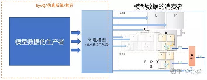
The environment model defines the boundary between the “producer” and “consumer” of model data. With this boundary, we can replace the implementation of the “model producer” on the left.

The domain controller that supports Level 3 intelligent driving integrates a hardware module for accelerating perception algorithms, which can complete the calculations required to build the environment model by itself. Alternatively, simulation software can be used as the producer of environment model data, so that functional development of the “model data consumer” on the right can commence directly even when algorithm capabilities are not yet available. This is also the significance of the environment model as a product boundary. Through product-level differentiation, different teams can complete their own professional product definitions. Different development teams can simultaneously carry out their own product development.

Environment Model Module and Interface Requirements

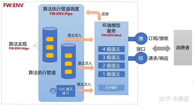
“Environment Model” can be provided as a service at the FW layer (FW:ENV:Mod). It stores real-time 1-4 level environment semantics and retains historical information for a period of time.

FW: ENV: Mod needs to provide a semantic injection interface whose format conforms to the environment model semantic specification and can support the injection of semantics at multiple different levels. FW: ENV: Pipe is the execution pipeline for environment model-related algorithms, responsible for assembling algorithm modules (FW: ENV: Algo) and providing the execution environment of algorithm modules. FW:ENV: Pipe will be injected into the FW:ENV:Mod service at an appropriate semantic generation.

ENV: Mod, ENV: Pipe, and ENV: Algo together form the FW:ENV module of the L.FW layer.

# FW:ENV Module Access Interface for Environmental Model

The FW:ENV module needs to provide access interface to the environmental model for consumers, in a format that executes multilevel semantics and supports the expression of real-world models. The interface needs to support both “push” and “pull” forms. The “interface” refers to the request-response interface, which can be optionally implemented in a RESTful format. Consumers need to first subscribe to the FW:ENV to use the “push” interface and receive a notification when data arrives. Or, combining both forms, the consumers can first subscribe and then actively call the “pull” interface to request data when notified by push.

Another important feature of the FW:ENV module is to dynamically adjust the assembly of algorithm execution pipelines based on current requirements for environmental model data from consumers. FW:ENV:Mod has all the necessary information on semantic requirements for the environment. This information can be fed back to FW:ENV:Pipe to adjust the assembly of algorithms.

FW:ENV Implementation and Upper-Level Interface

The L.FW layer includes two parts: real-time domain and performance domain. FW:ENV needs to be implemented in both domains. The implementation of the real-time domain may be simplified, mainly in the Pipe part, which may not have a clear Pipe form, but only exists as an independent Algo. Nevertheless, FW:ENV:Mod needs to exist in both real-time and performance domains and support data synchronization. For instance, the environmental semantic information published by the deep learning vision algorithm in the performance domain can be obtained by the planning algorithm running in the real-time domain. The reverse is also true. To avoid unnecessary data transmission, data that is not required by one domain can be unsynchronized. However, this is an optimization issue of transmission, and the basic data synchronization logic remains the same.

FW:ENV provides some interfaces and SDK for the upper-level L.APK layer:

• Environmental model semantic definition standard

• FW:ENV’s “push” and “pull” interface explanation and SDK

• Customized development instructions and SDK for FW:ENV:Pipe, supporting the L.APK layer to develop customized pipes.

• Customized development instructions and SDK for FW:ENV:Algo, supporting the L.APK layer to develop customized Algos that can be assembled into existing Pipes.

Deep Into the EPX-SA Model

The Abstract Semantics of EPX

EPX-SA is an abstract model that decomposes complex autonomous driving scenarios and provides a consistent way of expression. The following figure describes a three-layer cooperation of EPX. First, let’s define the symbol notation.

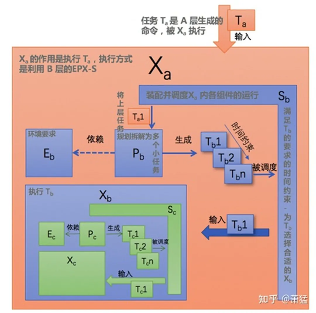Due to the fractal recursive nature of EPX identifiers, it is necessary to annotate their hierarchy in order to avoid ambiguity. We use subscripts to express the hierarchical level of the fractal recursion. Relative levels are denoted by numerical subscripts “-1” and “+1”, indicating the next layer and the previous layer, respectively. For example, E-1 denotes the E in the next layer and P+1 denotes the P in the previous layer. Absolutes levels are denoted by alphabetical subscripts, such as Xa, Xb, and Xc, representing the progressively increasing levels of X. Each group of EPXS is within X+1.

Let’s define the concept of EPX-S.

• E represents the perceptual requirements of the environment. When we have environment model services to provide perceptual capabilities, we do not need E to have actual perceptual capabilities, we only need to describe the perceptual requirements and not actually execute perceptual actions.

• P is the abstract planning that breaks down the task T+1 of the previous layer into a series of small task sequences (T1, T2, …, Tn), expressed as Seq (T), which is sent to S for scheduling. Seq (T) has a time-constraint property, which will be explained later in the text. P will replan new Seq (T) based on changes in E and will be rescheduled by S.

• S is an abstract scheduler. It has several functions:

1. Responsible for assembling all components within X+1.
2. Schedules the execution of each T in Seq (T) and needs to meet the time constraints of Seq (T). When the time constraints cannot be met, S needs to respond.
3. Selects the appropriate X for each T.

• Seq (T) is a task sequence generated by P. Here, a task is an abstract concept, representing a “certain goal that needs to be achieved under certain constraints”. Constraints may be applied to a single task T, such as requiring completion within a certain time or space, or to the task sequence Seq (T), such as requiring completion in a specific order or allowing certain tasks to be performed in parallel, which will introduce arbitration mechanisms.

• X is the executor in the same hierarchical layer as T. It either directly completes the actual task execution action or calls its internal lower layer E-1P-1X-1 to execute. Each time X completes a T, it notifies S. S will check if Seq (T) is empty. If not, it will execute the next T. If Seq (T) is empty, it will ask P to generate a new Seq (T). If P discovers based on information from E that T+1 has already been completed, it will output an empty task sequence and S will assume that X+1 has been completed.

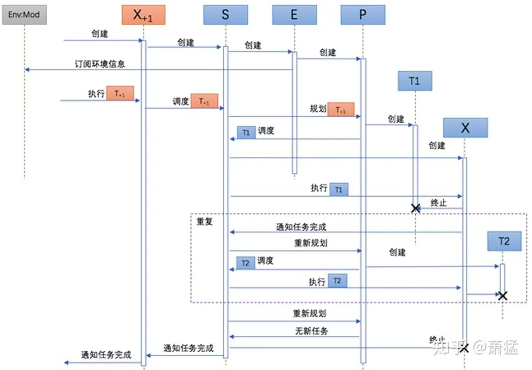
The following UML sequence diagram illustrates a typical process of EPX execution.- When X+1 is created, it first creates S internally, and then S creates E and P, and E subscribes to the required environmental information from the environment model service.

• T+1 is handed over to X+1 for execution by an external entity. It is scheduled by S and then handed over to P for planning.

• P creates task T1 and hands it over to S for scheduling. S creates X and hands T1 over to X for execution.

• X destroys T1 after completing the execution and notifies S of completion. S notifies P to replan.

• Steps 3 and 4 are repeated until P does not produce any new tasks, and S notifies that there are no new tasks.

• S notifies X+1 of task completion, and X+1 notifies the external entity.

The innermost X represents a very simple execution mechanism and does not need to be further divided into the next layer of EPX. This is equivalent to the termination condition of recursion.

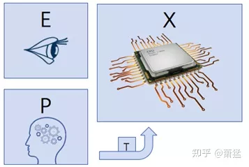
The outermost EPX is not always all part of the computer system. As shown in the figure above, human perception completes the work of E, the human brain completes the work of P, and the generated tasks T are handed over to the computer system X for execution. Therefore, for the computer system, X is the starting point of fractal recursion.

Example of EPX:

The setting and decomposition of OKR (Objectives and Key Results), a management tool and method for clear goal setting and tracking, were invented by Andy Grove, the founder of Intel Corporation. It was introduced to Google by John Doerr and was widely used in companies like Facebook, LinkedIn, etc. since 1999. OKR was introduced to China in 2014, and companies such as Baidu, Huawei, ByteDance, etc. have gradually used and promoted OKR since 2015. For more details, please refer to the relevant entries on Baidu Encyclopedia (baike.baidu.com/item/OKR).# Objectives and Key Results (OKR) of an Enterprise

The OKR of an enterprise is determined from the top down. Generally, the company sets several top-level objectives and key results (KRs) to achieve these goals. Then each department specifies its own OKR based on the company-level OKR, and each group within the department, from individuals to the top, determines its own OKR.

We can use the EPX model to explain OKRs. To understand the business status and data and analyze the market, the enterprise needs to perceive the market environment and its own status, which is the “E” part of the enterprise. Based on this perception, the enterprise conducts business analysis and planning, which is the “P” part, and the result of “P” is the company-level OKR (objectives and key results), which is the “T”. The “KR” (key results) can also be regarded as the “T”, and “O” is the grouping of “T”. The company’s leaders will assign the OKR to each business department to complete, and a certain department may only complete one or more “KRs”. In this case, each business department is “X”. It is the job of “S” to determine which department completes which “KR”.

When the business department (X) receives the “KR” (T) that it needs to complete, it analyzes (E-1) and plans (P-1) its own OKR (T-1) based on its own situation, and then hands it over to each group (X-1) in the department to further determine the next level of OKR. The functions of each group are different, and the types of T-1 that they can complete are also different, which is assigned by S-1.

The first level of the group is E-2X-2P-2, and each individual is E-3X-3P-3. This is not further decomposed.

The whole recursive decomposition process is the implementation of a complete EPX model. This process breaks down an abstract task layer by layer into concrete execution layers and completes it.

Adaptive Cruise Control (ACC)

As an advanced function of cruise control, the greatest advantage of ACC over regular cruise control is that it not only maintains the vehicle speed predetermined by the driver, but also adjusts the vehicle speed adaptively according to the state of the front vehicle, and even automatically brakes and starts at the appropriate time.

Several typical functions of ACC are:

(1) When there is no vehicle in front, the ACC vehicle will be in normal cruise driving state, traveling at the speed set by the driver, and the driver only needs to control the direction (lateral control).

(2) When a leading target vehicle appears in front of the ACC vehicle, if the speed of the target vehicle is less than that of the ACC vehicle, the ACC car will automatically begin to decelerate to ensure the distance between the two vehicles is at a safe distance, and follow the front car automatically at the same speed.

(3) When the front vehicle stops, the vehicle will also stop, wait for the front vehicle to start and then automatically accelerate to follow the front car.(4) For a better user experience, the driver can still interact with the ACC system to a limited extent while ACC is being activated. For example, the system will automatically stop when the vehicle is about to come to a fast stop, and “light stepping on the accelerator” notifies the ACC system to be ready to start at any time.

The general logic of ACC functionality can be represented as a state machine.

We use the EPX model to design the software architecture of the ACC function.

First, it is necessary to determine the recursive level of EPX.

As shown in the following figure, we divide the ACC’s EPX recursive level into four levels: level 0-3. E0 and P0 exist outside the system, X0 represents the ACC system, which can achieve adaptive cruise control function according to the user’s set speed. X0 has E1, P1, and X1. E1 includes requirements for the environment, such as vehicle information, lane information, and vehicle information. It needs to know whether there is a vehicle in front of the lane and the speed and distance of the vehicle in front, as well as the speed limit of the lane. P1 determines the speed that needs to be achieved within a certain period of time (0~ user set cruising speed) based on the information obtained from E1, and is executed by X1. E2 inside X1 is no longer relevant, and only needs to be concerned with the current vehicle speed. P2 calculates the acceleration to be achieved within a certain period of time and is executed by X2. Similarly, P2 inside X2 generates information on the throttle opening and is executed by X3. X3 can be the vehicle control unit (VCU). Here, X3 is regarded as the end point of recursion, which means that we consider the execution mechanism inside X3 to be transparent to us and the details are not necessary for ACC applications. Of course, there may be further EPX mechanisms inside X3, but we are not concerned with these here.

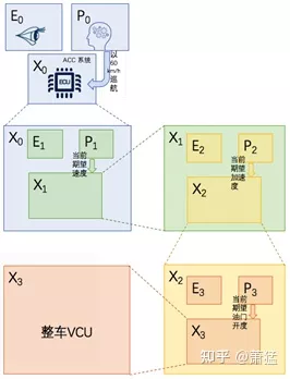
Through the four-level fractal recursion from 0 to 3, we simplify the problem step by step. It should be noted that X0 to X3 have different time cycles for their task execution.

X0 is a complete process of enabling ACC, and its time cycle can be more than 10 minutes.

X1 needs to make the car reach a certain speed. Generally, we expect this process to be completed within 10 seconds while ensuring safety and comfort.

X2 needs to make the car reach a certain acceleration. Generally, this is done within 200~1000 milliseconds.

X3 is to achieve the expected throttle opening, and its execution cycle may be in the range of 20~200 milliseconds.The execution times of X1, X2, and X3 are also dependent on the specific task granularity of their corresponding outputs P1, P2, and P3. Generally, PID control algorithm can be adopted for P1, P2, and P3, and the execution time of X is related to the increment interval of the algorithm implementation of the corresponding P. However, the magnitude of the execution time of X1, X2, and X3 decreases gradually. We need to determine whether a certain level of EPX must be executed in real-time domain based on this magnitude.

Another issue is where the ACC state machine mentioned earlier is reflected. There are two feasible ways.

The first is to implement all state machine logic in P1. P1 saves state changes and outputs different speed requirements based on different states. The second way is to introduce S1 and add multiple different implementations of P1. Multiple different implementations of P1 handle different scenarios in the state machine. Here, the scenario may be a state or a combination of multiple states. For example, some P1 processes the situation where there is no car in front, some P1 processes the situation where there is a car in front and it is decelerating, and some P1 processes the situation where there is a car in front and the car has stopped. S1 is responsible for selecting different P1 to be assembled into the processing flow based on the current situation. In this way, the state machine is actually distributed in S1 and different implementations of P1. This is another way to decompose the problem. The specific approach depends on the specific design, and the one that can better meet the actual situation and simplify the design should be used. A specific problem requires a specific analysis.

Arbitration Mechanism

As mentioned earlier, S can simultaneously start multiple parallel Xs to perform different tasks. As shown in the figure below:

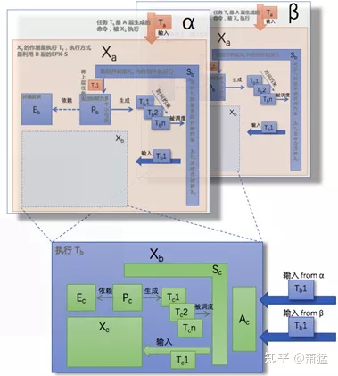
Alpha and beta are two parallel EPX execution mechanisms that are simultaneously started by the upper layer. However, at the Xb level, they both reference the same Xb instance. In this way, the Xb instance will receive execution requests from two different sources at the same time. This requires an arbitration mechanism to analyze inputs from multiple sources, and if there is no conflict, whether they can be merged. If there is a conflict, the execution with the highest priority should be selected.# Translation

The Lane Keeping Assist (LKA) function and Automatic Emergency Braking (AEB) function can work simultaneously with Adaptive Cruise Control (ACC) and have their own independent EPX fractal recursive structure. But at the innermost layer, X (pointing to VCU), the fractal recursive structure can be shared with ACC. The shared X needs an arbitration mechanism (A). Since LKA outputs steering torque for lateral control, it does not conflict with ACC’s longitudinal control and can generally be executed together. However, AEB also outputs longitudinal control signals, so it needs to be arbitrated with ACC’s output, but AEB generally has higher priority. The arbitration logic is implemented by component A.

Not all EPX hierarchical levels have component A. It is only required when EPX can be referred to multiple times. Component A knows the ability of this level, and is responsible for the arbitration logic of this EPX level.

The Significance of FW:ENV and FW:EPX-SA in Software Architecture

In Chapter 3, we mentioned that the L.FW layer began to have semantics related to intelligent driving, which mainly provides a software framework and basic components for intelligent driving. Section 4.1 pointed out that “L.FW does not implement specific algorithms, but it prepares the context for algorithm execution, including the resources, time, and data required for algorithm execution. It is the container for algorithm execution.” Therefore, the software architecture of the FW layer is to provide a good organization and operating environment for various intelligent driving-related algorithm operations. Let the algorithm focus on its own logical implementation, and let the framework handle the assembly and execution process.

FW:ENV and FW:EPX-SA are the two most important frameworks of the L.FW layer, which have the following important significance for the software architecture of the entire L.FW layer:

1. The FW:ENV framework provides a standardized semantic hierarchy for perception, which serves as the basis for building environmental models and defines standardized API interfaces for perception development, thus decoupling perception development from intelligent driving function development.

2. The FW:ENV framework provides a runtime environment for perception algorithms.

3. FW:EPX-SA provides a three-dimensional method for scenario analysis and simplification.

4. These two frameworks provide a consistent methodological model for the development of L1-L2 and L3 and above functionality.

5. It makes component-based development possible. Each Pipe in FW:ENV can be a collection of components, and each algorithm can also be a component. Each EPX hierarchical level in FW:EPX-SA can be a component, and each individual EPXSA in each level can also be a component. Based on the components for analysis, design, development, and testing, the development of this complex system can be broken down into manageable units, which is of great significance for the software development of intelligent driving systems.6. It supports a reuse mechanism for components. Components with clearly defined capabilities and data interfaces are reusable. On one hand, already well-tested components can be reused in different functions (or scenarios) within the same autonomous driving system. On the other hand, an accumulated library of reusable components can greatly accelerate the development of new projects.

6. In essence, it defines the API interface form for the application layer (L.APK).

Implementation of L.FW in the Domain Controller

Both real-time and performance domains need to implement ENV and EPX-SA frameworks

In the previous example of ACC, we mentioned that different EPX hierarchy levels have different time requirements for execution. The smaller the execution time cycle, particularly for X with deterministic time cycle requirements, should be completed in the real-time domain. Operations that are closer to the vehicle control layer should typically be implemented in the real-time domain. Certain perception algorithms, usually radar-related algorithms, will have real-time domain implementation requirements. This is because it requires precise control of the sending and sampling time of radar pulses, which generally have millisecond-level time requirements. We should implement our respective FW: ENV and FW: EPX-SA frameworks in both the real-time and performance domains, although the implementation methods can vary.

Data synchronization of environmental models

The environmental model data generated by the FW: ENV of the performance domain needs to be synchronized with the real-time domain. In other words, when the E in the real-time domain subscribes to environmental information in a certain EPX, it is actually generated in the performance domain, but E in the real-time domain only needs to subscribe to FW: ENV in the real-time domain. However, the required data will automatically synchronize from the performance domain to the real-time domain. As shown below:

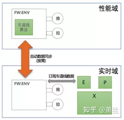
The real-time domain only needs to subscribe to FW: ENV to obtain lane data. As for how lane data is synchronized from the performance domain to the real-time domain, it is the responsibility of the FW: ENV in both domains to implement. At the same time, the data that needs to be synchronized between two domains should be sufficient and necessary, that is, irrelevant data (not subscribed by any E) should not be synchronized. Data synchronization is bidirectional, such as the vehicle status information is also part of the environmental model and is generally obtained from the real-time domain and synchronized to the performance domain as needed.

Similar data transmission between two domains is implemented in almost all intelligent driving systems that are divided into “real-time domain” and “performance domain”. So what is special about the data synchronization mechanism described in this article? There are three points:1. Structured expression and standardized definition of environment model semantics. We need to define a structured expression form of multi-level environment model semantics (using some Interface Definition Language (IDL) to describe) to form an internal standard. This structured standard is not designed for specific projects or specific intelligent driving functions, but should have some generality. Of course, there can be a gradual version evolution process.

2. The implementation mechanism of the environment model data synchronization between two domains is universal. Generally speaking, different projects will design project-specific transmission protocols for environment model data transmission between two domains. However, the data of the FW:ENV framework is not transmitted between two domains in this way. Because we have defined a standardized environment model semantic format, a specific project-independent universal implementation mechanism can be made. Even when the standard version changes, a universal template code should be able to be generated through code generation.

3. The runtime synchronization mechanism is automatic. Once the system is up and running, the synchronization of environmental model data between two domains is automatic. Environmental model data consumers in the real-time domain or performance domain do not need to know where the environmental model data is generated.

Proxy mode of X in EPX

Generally speaking, in the implementation of the EPX multilevel recursive model, the closer to the user interaction in the outer layer, the lower the real-time requirement, and it is mostly completed in the performance domain. As the layer goes deeper, the real-time requirement is high, and it is mostly completed in the real-time domain. That is to say, for the same EPX multilevel sequence, some will happen in the performance domain, and some will happen in the real-time domain. How to implement the cross-domain EPX multilevel recursion in this case?

The solution is to implement a real-time domain X proxy in the performance domain and assemble it into the EPX structure of the performance domain.

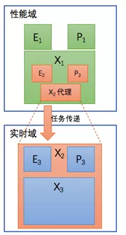
As shown in the figure above, X2 is the innermost and the terminating layer of the recursive structure of the performance domain’s EPX. However, in fact, X2 is only a proxy for an X structure in the outermost layer of the real-time domain. This proxy directly sends tasks to the X2 instance in the real-time domain for execution.

That is to say, in order for the X in the real-time domain to be used by the performance domain, a proxy for it needs to be implemented in the performance domain, which communicates across domains with the actual X instance. The same is true in reverse.

Technical selection reference for implementation solution

Strong dependency of L.FW on L.BSW# Development of L.FW layer requires building upon L.BSW layer. L.BSW provides the basic functionality required for automotive electronic controllers (ECU), as well as a runtime environment and basic services for L.FW. To utilize the execution mechanism provided by L.BSW, L.FW must be developed in accordance with its application development specification, code written according to its configuration standards, and APIs and services provided by L.BSW. This creates a strong dependency relationship between L.FW and L.BSW layers.

In real-time domain, L.BSW layer can be implemented using CP AutoSar or other RTOS (in some cases, real-time domain may also have multiple cores, with one core running CP AutoSar to handle vehicle interaction, and other cores using simpler RTOS to tackle partial computation). When using CP AutoSar, configuration for CP BSW layer is written, RTE is generated, and SWC is developed with RTE interface. If L.FW is implemented on this basis, it becomes closely related to CP AutoSar.

In performance domain, the same issue arises; if developed based on AP AutoSar, compliance with AP’s set of specifications is required, but with the added benefits brought by AP. Developing based on ROS2 uses a completely different approach and implementation architecture, utilizing ROS2 concepts such as Node, Topic, Service, and Action. However, developing different sets of L.FW layers for different L.BSW layers may make it possible for L.APK layer to be compatible with different L.BSW platforms, since the differentiated implementation of L.FW layer actually plays a role as an intermediate layer, shielding lower layers from differentiation.

Therefore, before developing L.FW layer in practice, it is necessary to first select the technical solution for the L.BSW layer.

This article is a translation by ChatGPT of a Chinese report from 42HOW. If you have any questions about it, please email bd@42how.com.