Introduction

In the previous issue of Introduction to Autonomous Driving Technology, we introduced the principles, formulas, and code writing of Kalman filters, using obstacle tracking as an example. In the following issues, we will continue to explore another important field of autonomous driving technology – computer vision.

In Introduction to Autonomous Driving Technology (V), “No Visual Sensor, No Autonomous Driving?” I introduced how on-board visual sensors can achieve lane line detection, obstacle detection, traffic sign recognition, drivable space detection, and traffic signal detection. All of these detection results rely on computer vision technology.

In this article, I will use the primary lane line detection project provided by Udacity’s Autonomous Driving Engineer degree program as an example to share the computer vision technology used in the course. The content includes the basic usage of the OpenCV library, as well as the computer vision technology used in lane line detection, including its basic principles and use effects, to help you gradually understand computer vision technology.

Main Content

Before introducing computer vision technology, let’s first discuss the input and output of this article.

Input

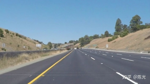
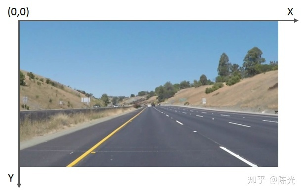
A road image taken by a camera, which needs to include lane lines, as shown in the following figure.

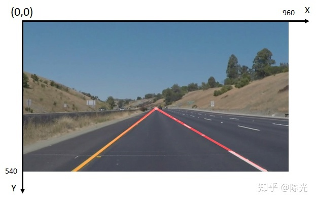
Output

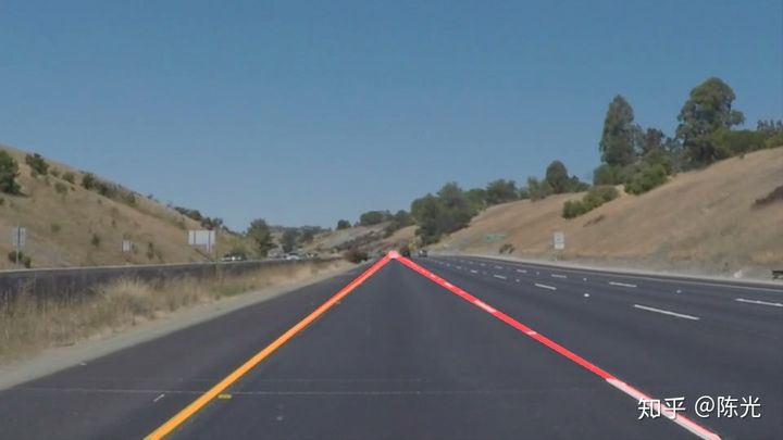
The straight line equations and effective distance of the left and right lane lines in the image coordinate system. The equations of the left and right lane lines should be drawn on the original image, as shown in the following figure.

After clearly defining the input and output, we will start using computer vision technology to process the original image step by step.

Original Image

Before understanding the image, let’s first review the physics knowledge learned in middle school – the three primary colors of light: red (Red), green (Green), and blue (Blue), which form visible light in different proportions. The following figure shows this.

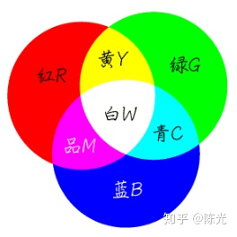
Picture from: https://zhidao.baidu.com/question/197911511.html

Each pixel in the image is composed of three color channels – RGB (red, green, blue). To facilitate the description of the RGB color model, each channel in the computer is constrained to a range of 0-255, from dark to light.When the R channel value of a pixel is 255, and the G and B channel values are 0, the resulting color is the brightest red. When all three RGB channels have a value of 255, the color represented is the brightest white. When all three RGB channels have a value of 0, the color displayed is the darkest black. In the RGB color model, there is no combination brighter than [255, 255, 255].

Based on this theoretical foundation, a color image is actually composed of three single-channel images overlaid, as shown below.

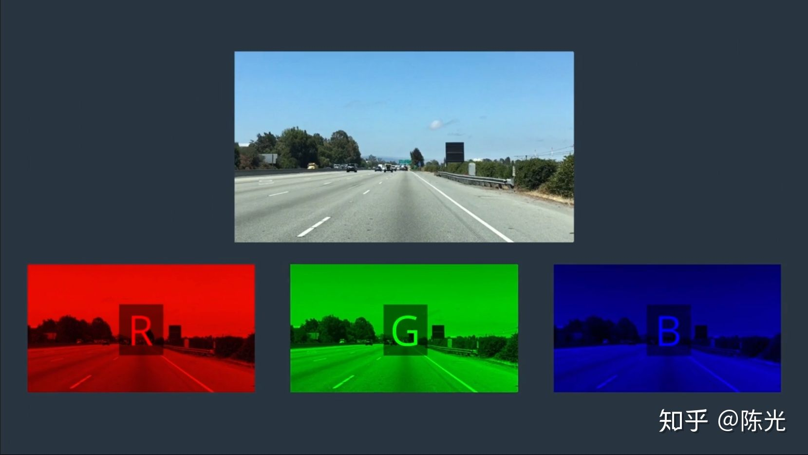
Image source: Udacity Autonomous Vehicle Engineer degree program

Taking OpenCV based on Python as an example, the code for reading an image named test_img.jpg into computer memory is as follows:

import cv2
img = cv2.imread('image_name.jpg')

After reading the image, we can see the image as a two-dimensional array, with each array element storing three values, corresponding to the values of the RGB channels.

OpenCV defines that the origin (0, 0) of the image is in the upper left corner of the image, with the X-axis to the right and the Y-axis down, as shown in the figure below.

It should be noted that because early developers of OpenCV are accustomed to using the BGR-ordered color model, the pixels read by OpenCV’s imread() function are arranged in BGR, not the common RGB. Therefore, attention should be paid when writing the code.

Grayscale processing

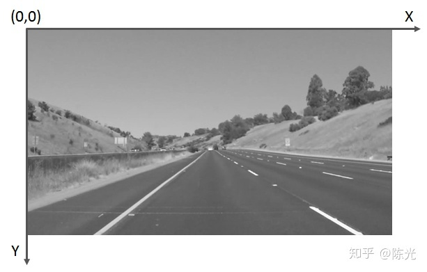
Considering that it is more complicated to process data from three channels, we first convert the image to grayscale. The process of grayscale conversion is to unify the RGB values of each pixel. The grayscale image will change from three channels to one channel, which will make it much easier to process.

Usually, this value is obtained by calculating weighted average of RGB channels. The human eye has different sensitivities to RGB colors, which is most sensitive to green, with a relatively high weighting, and least sensitive to blue, with a relatively low weighting. The specific calculation formula for grayscale transformation of the pixel point at coordinates (x, y) is as follows:

Use the cvtColor() function provided in OpenCV to easily perform grayscale processing on images.

gray = cv2.cvtColor(img, cv2.COLOR_BGR2GRAY)

Since the data arrangement of img read by cv2.imread() is in BGR, the parameter used here is BGR2GRAY.

The grayscale processed image is shown below:

Edge Extraction

In order to highlight the lane lines, we perform edge processing on the grayscale image. “Edges” are areas in the image where there is a sharp contrast between light and dark. Lane lines are usually white or yellow, while the ground is usually gray or black, so there will be a sharp contrast at the edges of the lane lines.

Common edge extraction algorithms include Canny algorithm and Sobel algorithm, which only differ in their calculation methods but achieve similar results. You can choose the algorithm based on the actual image you want to process. Choose the one that achieves better results.

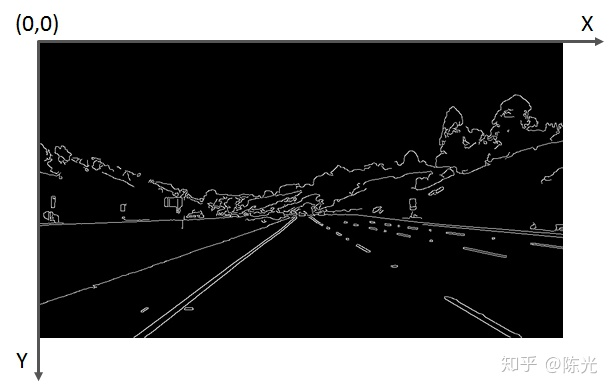
Taking the Canny algorithm as an example, after selecting specific thresholds, the edge extraction effect can be obtained by processing the grayscale image.

lowthreshold = 40
highthreshold = 150

cannyimage = cv2.Canny(gray, lowthreshold, high_threshold)

ROI Selection

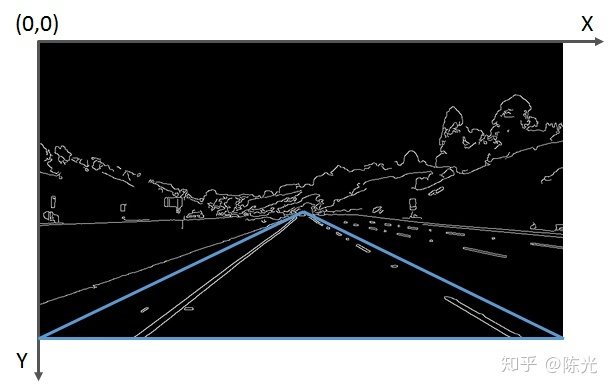
After edge extraction is completed, the lane lines to be detected are highlighted. In order to detect the lane lines of the lane where the vehicle is located, we need to extract the Region of Interest (ROI). The simplest way to extract the ROI is to “capture” it.

First, select a Region of Interest, such as the blue triangular area shown below. Traverse the coordinate values of each pixel point, if the current point is not within the triangular area, then the pixel of the point will be painted “black”, that is, the pixel value of the point will be set to 0.

To achieve cropping function, a regionofinterest function is defined by encapsulating some of the OpenCV functions, as follows:

def region_of_interest(img, vertices):

    # Define a mask with same size as the input image, which is also called a mask.
    # Introduction to masks can be found here: https://www.cnblogs.com/skyfsm/p/6894685.html
    mask = np.zeros_like(img)   

    # Determine the ignore_mask_color based on the number of channels of the input image
    if len(img.shape) > 2:
        channel_count = img.shape[2]  # i.e. 3 or 4 depending on your image
        ignore_mask_color = (255,) * channel_count
    else:
        ignore_mask_color = 255

    # Fill in the polygon enclosed by [vertices], 
    # and retain the mask pixels inside the polygon
    cv2.fillPoly(mask, [vertices], ignore_mask_color)

    # Do the AND (bitwise) operation with mask to get only the portion of the image within the polygon
    masked_image = cv2.bitwise_and(img, mask)

    return masked_image

The interested region is then input to the function to extract the cropped edge image.

# Image pixel rows = canny_image.shape[0]  540 rows
# Image pixel columns = canny_image.shape[1]  960 columns

left_bottom = [0, canny_image.shape[0]]
right_bottom = [canny_image.shape[1], canny_image.shape[0]]

“`markdown
apex = [cannyimage.shape[1]/2, 310]
vertices = np.array([leftbottom, rightbottom, apex], np.int32)
roiimage = regionofinterest(canny_image, vertices)

The cropped image is shown below:

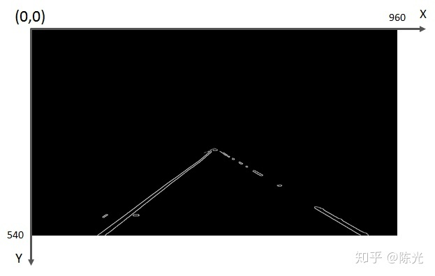
Hough Transform

After grayscale processing, edge detection, and region of interest cropping, we finally extracted the left and right lane lines from the complex image. Next, we use the Hough Transform to extract the straight lines (segments) from the image.

The Hough Transform is a feature detection method. Its principles and derivation process can be found in the classic Hough Transform.

Using the Hough Transform in an image can not only identify straight lines in the image, but also identify circles, ellipses, and other features in the image. OpenCV provides us with a function for detecting straight lines using the Hough Transform, which can detect line segments of different lengths by setting different parameters. Since lane lines may be dashed, the length of the detected line segments cannot be set too long, otherwise short line segments may be ignored.

The usage of the OpenCV Hough Transform line detection function is as follows:

rho = 2 # distance resolution in pixels of the Hough grid
theta = np.pi/180 # angular resolution in radians of the Hough grid
threshold = 15     # minimum number of votes (intersections in Hough grid cell)
min_line_length = 40 #minimum number of pixels making up a line
max_line_gap = 20    # maximum gap in pixels between connectable line segments
# Detect line segments using Hough Transform. The coordinates of the two endpoints of each line segment are stored in 'lines'.

“`
The code in Chinese Markdown:

lines = cv2.HoughLinesP (roi_image, rho, theta, threshold, np.array ([]),
                            min_line_length, max_line_gap)


封装一个绘图函数，实现把线段绘制在图像上的功能，以实现线段的可视化

def draw_lines (img, lines, color=[255, 0, 0], thickness=2):
    for line in lines:
        for x1,y1,x2,y2 in line:
            cv2.line (img, (x1, y1), (x2, y2), color, thickness) # 将线段绘制在 img 上


将得到线段绘制在原始图像上

import numpy as np
line_image = np.copy (img) # 复制一份原图，将线段绘制在这幅图上
draw_lines (line_image, lines, [255, 0, 0], 6)


结果如下图：

![霍夫变换直线检测](https://upload.42how.com/article/image_20210221234831.png)

可以看出，虽然右车道线的线段不连续，但已经很接近我们想要的输出结果了。



### 数据后处理



霍夫变换得到的一系列线段结果跟我们的输出结果还是有些差异。为了解决这些差异，需要对我们检测到的数据做一定的后处理操作。



实现以下两步后处理，才能真正得到我们的输出结果。



计算左右车道线的直线方程
根据每个线段在图像坐标系下的斜率，判断线段为左车道线还是右车道线，并存于不同的变量中。随后对所有左车道线上的点、所有右车道线上的点做一次最小二乘直线拟合，得到的即为最终的左、右车道线的直线方程。

计算左右车道线的上下边界
考虑到现实世界中左右车道线一般都是平行的，所以可以认为左右车道线上最上和最下的点对应的 y 值，就是左右车道线的边界。


基于以上两步数据后处理的思路，我们重新定义 draw_lines () 函数，将数据后处理过程写入该函数中。

The code in English Markdown:

```
lines = cv2.HoughLinesP(roi_image, rho, theta, threshold, np.array([]), min_line_length, max_line_gap)


Define a drawing function that draws lines on the image to visualize line segments:

def draw_lines(img, lines, color=[255, 0, 0], thickness=2):
    for line in lines:
        for x1,y1,x2,y2 in line:
            cv2.line(img, (x1, y1), (x2, y2), color, thickness) # draw the line segments on img


Draw the detected line segments on the original image:

import numpy as np
line_image = np.copy(img) # Make a copy of the original image to draw the line segments on
draw_lines(line_image, lines, [255, 0, 0], 6)


The resulting image is shown below:

![Hough Transform Line Detection](https://upload.42how.com/article/image_20210221234831.png)

As we can see, although the line segments of the right lane are not continuous, the output is already very close to what we want.



### Data Post-processing



The line segments obtained by Hough transform still have some differences from our desired output. To solve these differences, some post-processing operations need to be performed on the detected data.



Implement the following two post-processing steps to get our desired output:



Calculate the straight-line equation of the left and right lanes
Based on the slope of each line segment in the image coordinate system, determine whether the line segment is the left lane or the right lane and store it in a different variable. Then, perform a least-squares straight line fitting on all points on the left lane and all points on the right lane to obtain the final straight-line equation for the left and right lanes.

Calculate the upper and lower boundaries of the left and right lanes
Considering that in the real world, the left and right lanes are generally parallel, so it can be assumed that the y-values corresponding to the highest and lowest points on the left and right lanes are the boundaries of the left and right lanes, respectively.


Based on the strategy of data post-processing described above, we redefine the draw_lines() function and write the data post-processing process into the function.

“`

Function: draw_lines (img, lines, color=[255, 0, 0], thickness=2):

left_lines_x = []
left_lines_y = []
right_lines_x = []
right_lines_y = []
line_y_max = 0
line_y_min = 999
for line in lines:
    for x1,y1,x2,y2 in line:
        if y1 > line_y_max:
            line_y_max = y1
        if y2 > line_y_max:
            line_y_max = y2
        if y1 < line_y_min:
            line_y_min = y1
        if y2 < line_y_min:
            line_y_min = y2
        k = (y2 - y1)/(x2 - x1)
        if k < -0.3:
            left_lines_x.append (x1)
            left_lines_y.append (y1)
            left_lines_x.append (x2)
            left_lines_y.append (y2)
        elif k > 0.3:
            right_lines_x.append (x1)
            right_lines_y.append (y1)
            right_lines_x.append (x2)
            right_lines_y.append (y2)
<!-- Minimize the least squared line -->

“““markdown
leftlinek, leftlineb = np.polyfit(leftlinesx, leftlinesy, 1)
rightlinek, rightlineb = np.polyfit(rightlinesx, rightlinesy, 1)

Calculate corresponding x values based on line equation and max/min y values

cv2.line(img,
(int((lineymax – leftlineb)/leftlinek), lineymax),
(int((lineymin – leftlineb)/leftlinek), lineymin),
color, thickness)
cv2.line(img,
(int((lineymax – rightlineb)/rightlinek), lineymax),
(int((lineymin – rightlineb)/rightlinek), lineymin),
color, thickness)

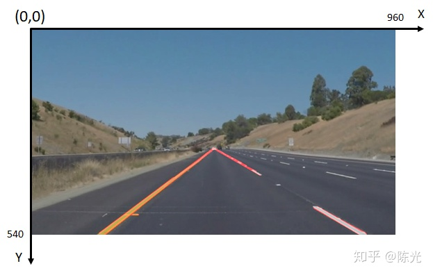
After post-processing the line segments, we can obtain the slope, intercept, and effective length of the two lines that meet the output requirements. The post-processed results are then plotted on the original image as shown below:

Processing Videos

Videos are actually continuous frames of images. Using a video-reading library, we can extract each frame of the video and apply the lane detection algorithm discussed above. We can then piece together the resulting images to form the final lane-annotated video.

The lane detection algorithm applied to a video is demonstrated in the following video:

Lane Detection with Introduction to Self-driving Technology

From the video, it can be seen that when the car is moving downhill, the front of the car tilts, causing changes in the area of interest and thus affecting the effective length detected. Therefore, this algorithm needs to be optimized for bumpy scenarios.

Conclusion

That’s all for the content of “Introduction to Beginner Lane Detection for Images”. For more information about this project, you can listen to the homepage trial of Udacity’s Self-driving Engineer program. We recommend that readers learn this first-hand.

During the actual writing of the lane detection code, you will find that many parameters need to be adjusted in each step to meet the processing requirements of subsequent algorithms. Therefore, this algorithm cannot be applied well to scenes with different lighting conditions and has poor robustness. In addition, due to the flaws of Hough Transform, it cannot detect curved lanes well.

Therefore, this algorithm is not well-designed. To develop a lane detection algorithm that can adapt to more scenarios, more advanced algorithms need to be used, which will be introduced in the next episode, “Advanced Lane Detection”.

Alright (^o^)/~, that’s all for this sharing. See you in the next episode~

This article is a translation by ChatGPT of a Chinese report from 42HOW. If you have any questions about it, please email bd@42how.com.