Preface
In “Introduction to Autonomous Driving Technology (13): Step by Step Guide to Writing Kalman Filters,” we used the example of a constant speed car model to help readers understand the basic principles of Kalman filters intuitively. It involves two processes: prediction and measurement update. The alternating execution of prediction and measurement update realizes the closed-loop of Kalman filtering in state estimation.
Subsequently, from the perspective of rational analysis, we used the data of obstacle position measured by lidar in unmanned driving as an example, combined with the formulas used in Kalman filtering, and used C++ and the matrix operation library Eigen to step by step implement the prediction and measurement update of Kalman filter.
In this sharing, we will use the sensor fusion project provided in Udacity’s Autonomous Driving Engineer Degree as an example to introduce how to use Extended Kalman Filters to solve the problem of tracking millimeter-wave radar targets. Because the content of this session is the advanced content of Kalman filters, it is recommended that readers first read “Introduction to Autonomous Driving Technology (13): Step by Step Guide to Writing Kalman Filters” to understand the formulas and meanings of the prediction and measurement update, and then read this article.
Content
Millimeter-wave Radar Data
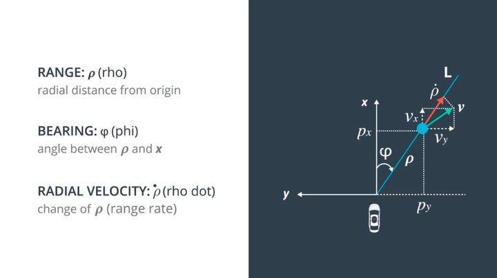
The way millimeter-wave radar observes the world is different from that of lidar. The principle of lidar measurement is the straight propagation of light, so it can directly obtain the distance of obstacles in the x, y, and z directions under the Cartesian coordinate system when measuring; while the principle of millimeter-wave radar is the Doppler effect, and the data it measures are all in the polar coordinate system.
As shown in the following figure, millimeter-wave radar can measure the distance ρ, the direction angle ϕ, and the rate of change of distance (radial velocity) ρ’ of obstacles from the radar in the polar coordinate system.
The measurement principle and more detailed data introduction of millimeter-wave radar can refer to “Introduction to Autonomous Driving Technology (7): Essential Millimeter-wave Radar for Mass Production”.
Theory of Extended Kalman Filter
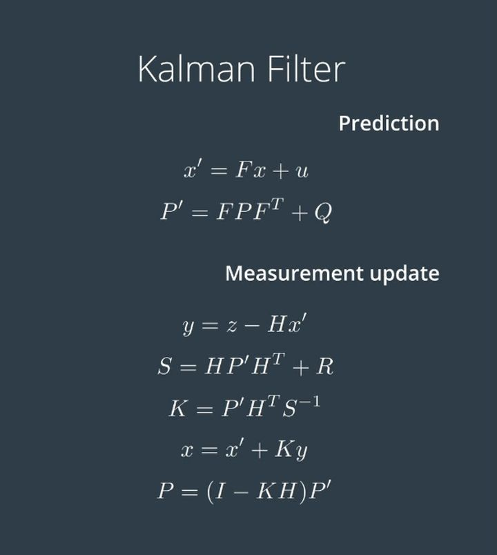
Once again, we use the precious wealth left by Mr. Kalman, that is, the seven formulas used in prediction and measurement update when estimating states, as shown in the figure below. The theory and programming of Extended Kalman Filters still need to use these formulas, which are only different in some places compared with the native Kalman Filters.
 ### Code: Initialization
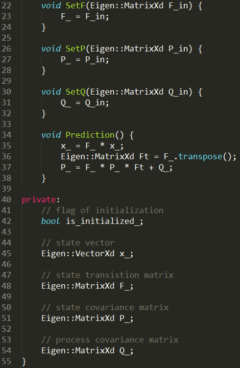
The process of completing the Extended Kalman Filter C++ code is essentially to combine the above formulas and complete the initialization, prediction, and observation step by step. Since the formulas involve a large number of matrix transpose and inversion operations, we use the open source matrix operation library Eigen to assist in our code writing.
As shown below, we have created a new class called ExtendedKalmanFilter, defined a state vector called x_. The VectorXd in the code represents a column vector of X dimensions, and the data type of the elements is double, which is used to ensure the compatibility of the code with different state vectors.
class ExtendedKalmanFilter {
    VectorXd x_;
    MatrixXd P_;
    MatrixXd F_;
    MatrixXd Q_;
    MatrixXd H_;
    MatrixXd R_;
    MatrixXd I_;
public:
    // Constructor
    ExtendedKalmanFilter() : x_(VectorXd()), P_(MatrixXd()), F_(MatrixXd()), Q_(MatrixXd()), H_(MatrixXd()), R_(MatrixXd()), I_(MatrixXd()) {}

    // Destructor
    virtual ~ExtendedKalmanFilter() {}

    // Initialize state vector x with input x_in
    void Init(VectorXd& x_in, MatrixXd& P_in, MatrixXd& F_in,
              MatrixXd& Q_in, MatrixXd& H_in, MatrixXd& R_in);

    // Execute Kalman Filter Prediction step
    void Predict();

    // Execute Kalman Filter Update step
    void Update(const VectorXd &z);

    // Get current state vector x
    const VectorXd &GetState() { return x_; }
};
When initializing the Extended Kalman Filter, various variables need to be set. For different motion models, the state vector is different. To ensure the compatibility of the code with different state vectors, we use the variable-length data structure in the Eigen library.
// Initialize state vector x with input x_in
void ExtendedKalmanFilter::Init(VectorXd& x_in, MatrixXd& P_in, MatrixXd& F_in,
                                 MatrixXd& Q_in, MatrixXd& H_in, MatrixXd& R_in) {
    x_ = x_in;
    P_ = P_in;
    F_ = F_in;
    Q_ = Q_in;
    H_ = H_in;
    R_ = R_in;

    I_ = MatrixXd::Identity(x_.size(), x_.size());
}
To initialize the Extended Kalman Filter, an initial state variable x_in is required, which represents the initial position and velocity information of the obstacle and is generally directly obtained from the first measurement results.
Code: Prediction
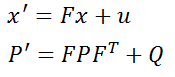
After completing the initialization, we begin writing the Prediction part of the code. First is the formula
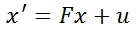
Here, x is the state vector, multiplied by a matrix F on the left, plus external influence u, to obtain the predicted state vector x’. Here, F is called the state transition matrix. Taking 2D uniform motion as an example, here x is
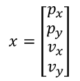
According to the formula learned in secondary school physics, s1 = s0 + vt, the predicted state vector after time △t should be
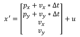
For the 2D uniform motion model, the acceleration is 0, and it does not affect the predicted state, so
 If it is changed to an acceleration or deceleration motion model, the acceleration ax and ay can be introduced. Here, u in s1 = s0 + vt + at^2/2 will become:
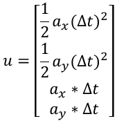
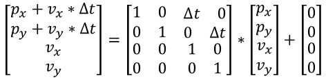
As an introductory course, we won’t discuss too complicated models, so the formula will be:

Finally, it will be written as:
Looking at the second formula of the prediction module:
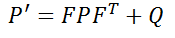
In this formula, P represents the degree of uncertainty of the system. This degree of uncertainty will be large when the Kalman filter is initialized. As more and more data is injected into the filter, the degree of uncertainty will decrease. The professional term for P is state covariance matrix. Q here represents process noise covariance matrix, which is the noise that cannot be expressed by x’=Fx+u, such as sudden uphill driving of the vehicle. This impact cannot be estimated by the previous state transition equation.
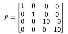
The millimeter wave radar measures the position and velocity of obstacles in the radial direction relatively accurately, with low uncertainty. Therefore, the state covariance matrix P can be initialized as follows:
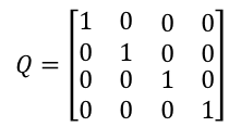
Since Q has an impact on the whole system but it’s uncertain how much impact it has on the system, for simple models, we can use the identity matrix or null value directly for calculation, that is:
Based on the above content and formula:
We can write the code for the prediction module.Translate the Markdown Chinese text below to English Markdown text, in a professional way. Retain the HTML tags inside the Markdown, and only output the result
Code: Measurement
The first formula for measurement is
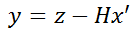
The purpose of this formula is to calculate the difference y between the observed value z and the predicted value x’.
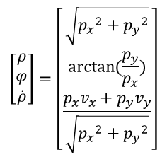
As mentioned earlier, the data characteristics of the millimeter-wave radar observed value z are shown in the figure below:

As shown in the figure, the data dimension of z is 3×1. To perform matrix operation, the data dimensions of y and Hx’ are also 3×1.
Using basic mathematical operations, we can complete the coordinate transformation from Cartesian coordinates to polar coordinates of the predicted value x’, and obtain Hx’. Then we calculate the difference between z and Hx’. It should be noted that in the step of calculating y, we bypass the calculation of the unknown rotation matrix H through coordinate transformation, and directly obtain the value of Hx’.
To simplify the expression, we use px, py, vx, and vy to represent the predicted position and velocity as follows:
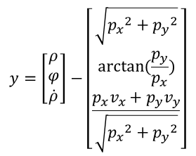
Since the measured value z and the predicted position x’ are both known, it is easy to calculate the difference y between them.
The conversion of millimeter-wave radar between Cartesian coordinates and polar coordinates involves the position and velocity transformation of the two coordinate systems, which is non-linear. Therefore, when dealing with non-linear models such as millimeter-wave radar, we write the formula for calculating y as:
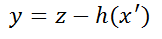
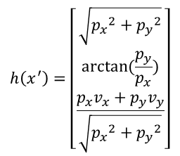
Following the above equation, h (x’) is:
 ## The Next Two Equations of Kalman Filter
The two equations below are used to calculate a very important parameter in the Kalman filter called Kalman gain K, which determines the weight of the difference y. The R in the first equation represents the measurement covariance matrix, indicating the difference between the measured value and the true value. Generally, the manufacturer of the sensor will provide this matrix. If not, we can obtain it through testing and debugging. S is a temporary variable used to simplify the equation.
Since calculating the Kalman gain K requires the measurement matrix H, the next task is to get H.
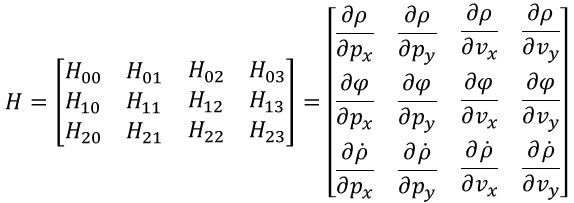
The observation z of the millimeter wave radar is a 3×1 column vector containing position, angle, and radial velocity, and the state vector x' is a 4×1 column vector containing position and velocity information. According to the equation y=z-Hx', we know that the dimension of the measurement matrix H is 3 rows and 4 columns, as shown below:
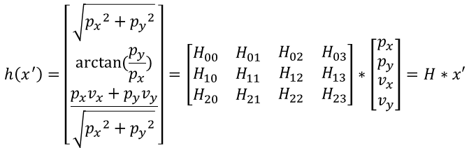
From the above equation, it is easy to see that the transformation on both sides of the equation is nonlinear, and there doesn’t exist a constant matrix H that can make both sides of the equation hold.
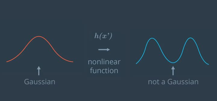
If a Gaussian distribution is used as the input and inputted into a nonlinear function, the result will no longer follow a Gaussian distribution, which will cause the Kalman filter equation to not be applicable. Therefore, we need to transform the above nonlinear function into an approximately linear function for solution.
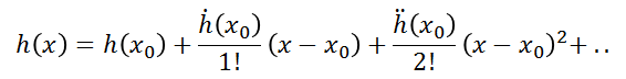
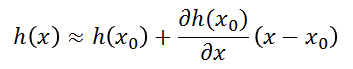
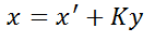
In the university course “Advanced Mathematics”, we learned that a nonlinear function y=h(x) can be expanded into a Taylor series at point (x0, y0) using the Taylor formula:
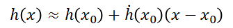
Ignoring the higher-order terms above quadratic, we can obtain an approximate linear equation to replace the nonlinear function h(x), namely:Translate the following Markdown Chinese text to English Markdown, in a professional way while keeping the HTML tags within the Markdown, and only output the result:
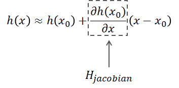
Expanding the nonlinear function h(x) to multiple dimensions means finding the partial derivative of each variable, i.e.:
The term corresponding to taking the partial derivative of x is called the Jacobian.
If we match the formula for taking partial derivatives with the formula we previously derived and look at the coefficient of x, we find that the measurement matrix H is actually the Jacobian expression in the Taylor formula.
Those who are interested in the process of deriving the Jacobian for multiple dimensions can study it themselves. Here, we will use its conclusion directly:
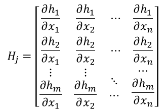
Obtaining the first-order partial derivatives of the nonlinear function h(x’) with respect to px, py, vx, and vy, and arranging them in a matrix, we finally get the Jacobian matrix H.
Where
Next, it is time to test your proficiency in partial derivatives in advanced mathematics!
After a series of calculations, the final measurement matrix H is obtained as follows:
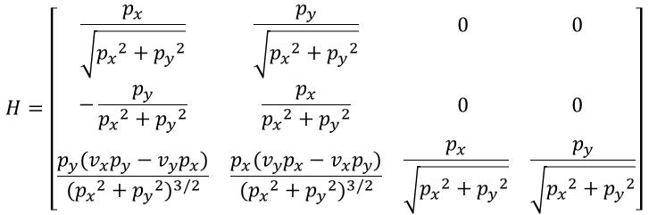
According to the above formula, after each prediction of the obstacle’s state, the corresponding measurement matrix H needs to be calculated based on the predicted position and velocity. This measurement matrix is the result of taking the derivative of the nonlinear function h(x’) at the position of x’.
Looking back at the last two formulas for the Kalman filter:
 The two equations actually complete the closed loop of the Kalman filter. The first equation updates the current state vector x, taking into account not only the predicted value from the previous time step, but also the measurement value and the system noise. The second equation updates the uncertainty P of the system based on the Kalman gain K, which is used for the calculation in the next cycle. The I in this equation is a unit matrix with the same dimension as the state vector.
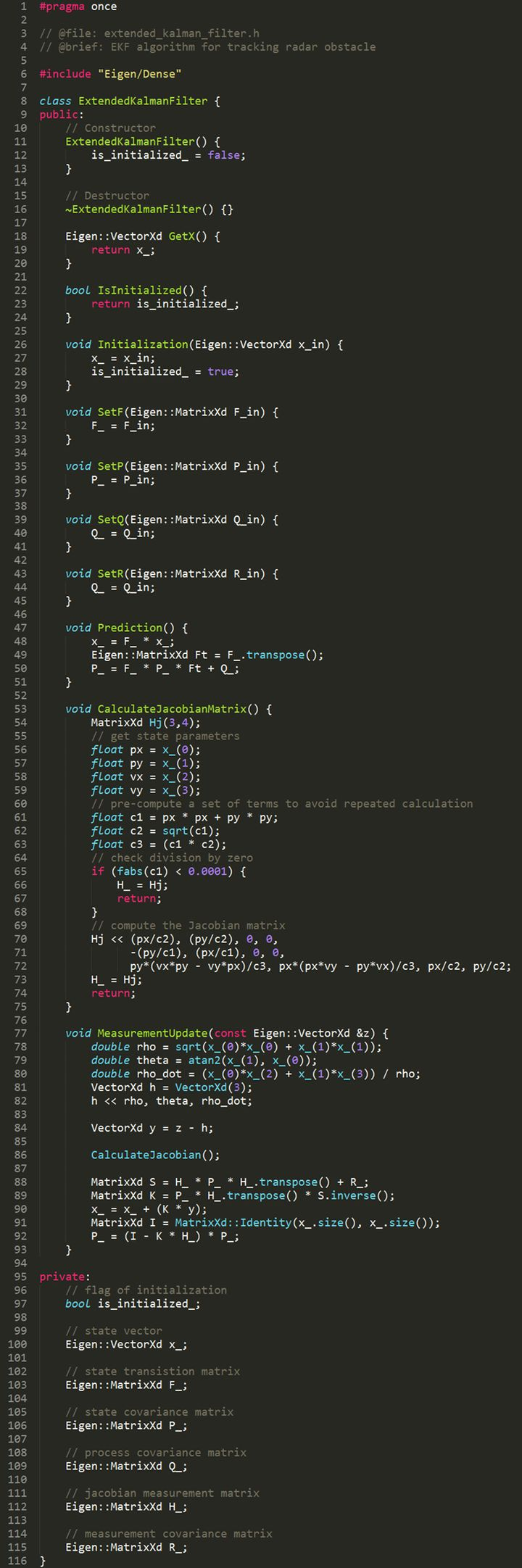
After completing the above derivation, we write the process into code as shown below, which is the embryo of an extended Kalman filter:
To demonstrate the use of the extended Kalman filter, here’s an example tracking obstacle data from a millimeter wave radar:
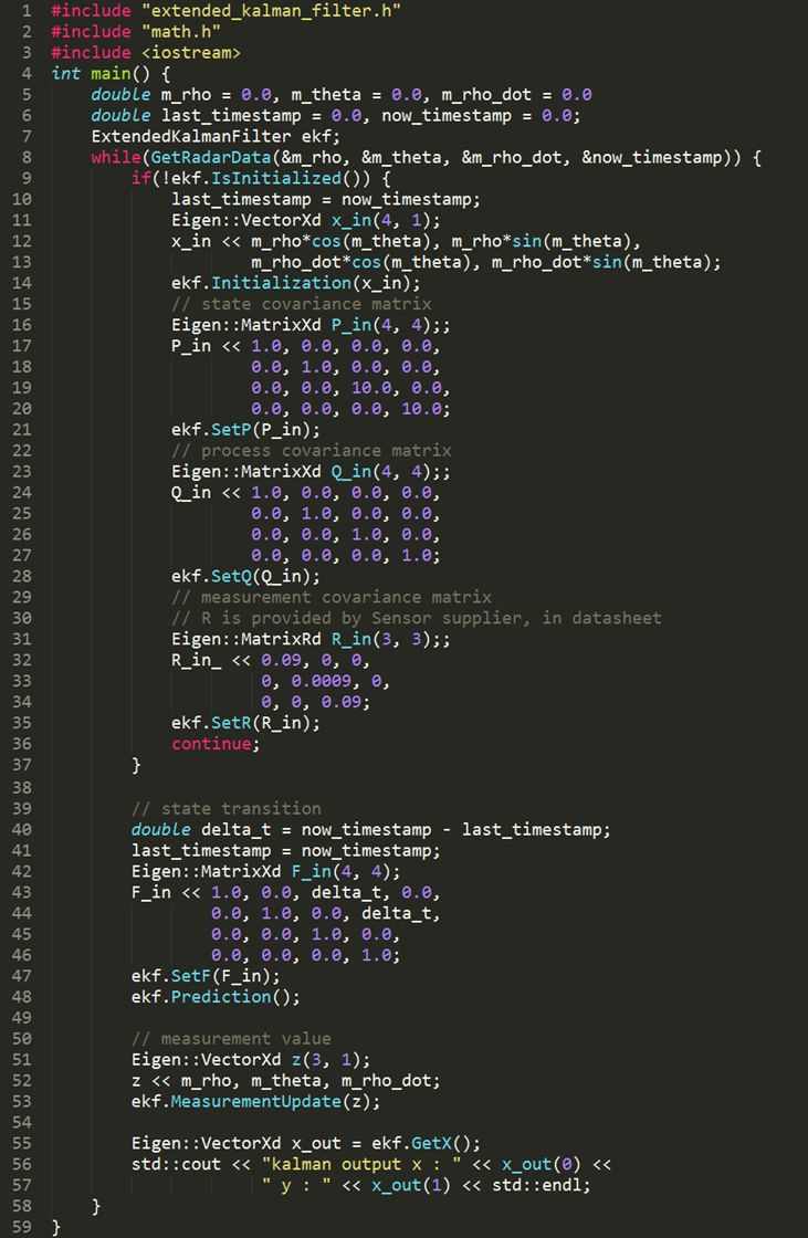
The GetRadarData function not only retrieves the distance, angle, and radial velocity of the millimeter wave radar obstacle data, but also retrieves the timestamp of the information collection to calculate the time difference between the previous and current frames delta_t.
The difference between the Extended Kalman Filter (EKF) and the classical Kalman Filter (KF) lies in the calculation of the measurement matrix H. EKF truncates the Taylor expansion of the nonlinear function after linearizing it to first-order, ignoring the remaining higher-order terms, thereby completing the approximate linearization of the nonlinear function. It is precisely because some of the higher order terms are ignored that the state estimation of EKF will lose some accuracy.
As long as you can apply the 7 classic equations of the Kalman filter to write the F, P, Q, H, and R matrices of the model, any state tracking problem will be easily solved.
To summarize, this is the entire process of the derivation of the Extended Kalman filter formula and the coding implementation. You will find that in actual engineering development, in addition to basic coding skills, theoretical knowledge from “Advanced Mathematics” and “Linear Algebra” is also essential. In the next article, I will combine classical Kalman filtering and the extended Kalman filtering to implement fusion with lidar data and millimeter wave radar data.
The derivation of the formulas and code implementation in this article are based on the content of the Udacity Self-Driving Car Engineer Nanodegree, and I recommend students who want to learn more details to enroll in the program. I have an invitation code worth ¥320: 50C3D1EA.Alright (^o^)/~, that’s all for this sharing.
This article is a translation by ChatGPT of a Chinese report from 42HOW. If you have any questions about it, please email bd@42how.com.