
Author: Wei Yin
The TOPS competition for autonomous driving has practical significance, but its significance is not as great as imagined, and there are many misconceptions. Failure to properly recognize these misconceptions can easily lead to undesirable consequences.
TOPS only means GPU computing power
Firstly, the value of computing power is related to the chip you are using. If your algorithm mainly involves scalar calculation, then this value is meaningless. Currently, when we say TOPS high computing power, we actually mean the computing power for GPU matrix multiplication and accumulation.
Different chips are connected to the outside world through buses and have their own cache systems and digital and logical computing units. The difference between CPU and GPU lies in the structural differences of their cache systems and digital logical computing units. Although CPU has multiple cores, their total number is not more than two digits. Each core has a sufficiently large cache and sufficient digital and logical computing units, and is assisted by many hardware accelerators, including much faster branch judgments and even more complex logical judgments. The number of cores in a GPU far exceeds that of a CPU and is known as a “multi-core” processor (NVIDIA Fermi has 512 cores). Each core has a relatively small cache size and fewer and simpler digital logical computing units (initially, GPUs were weaker than CPUs in floating-point calculation). As a result, CPUs are good at processing computing tasks with complex calculation steps and complex data dependencies, such as distributed computing, data compression, artificial intelligence, physical simulation, and many other computing tasks.
When programmers write programs for CPUs, they tend to optimize algorithms through complex logical structure and reduce the running time of computing tasks, i.e., Latency. When they write programs for GPUs, they use its advantages in processing massive amounts of data to increase the overall data throughput (Throughput) to cover Latency.
In general, CPUs are used for scalar calculations, mainly for path planning and decision-making algorithms. In addition, some laser radar uses ICP point cloud registration algorithm, which CPUs are better equipped to handle than GPUs. The commonly used sensor fusion algorithm, such as Kalman filtering algorithm, is also mostly scalar calculation. GPUs are used for vector or, more precisely, vector calculations, including point clouds, maps, deep learning, and the core is matrix computation. We can regard scalar as a zero-order tensor, vector as a first-order tensor, and matrix as a second-order tensor.
Currently, the physical computing unit for TOPS is the Multiply Accumulate (MAC) operation, which is a special operation in a microprocessor. The hardware circuit unit that implements this operation is called a “multiplying accumulator”. This operation is to add the product of multiplication b x c and the value of accumulator a, and then store it in the accumulator a:
 The program may need two instructions if MAC commands are not used, but many operations (such as convolution operation, dot product operation, matrix operation, digital filter operation, and even polynomial evaluation operation) can be decomposed into several MAC instructions, thus improving the efficiency of these operations.
The input and output data types of MAC instructions can be integers, fixed-point numbers, or floating-point numbers. When processing floating-point numbers, there will be two rounds of rounding, which is common in many typical DSPs. If a MAC instruction only has one rounding when processing floating-point numbers, this type of instruction is called “fused multiply-add” (FMA) or “fused multiply-accumulate” (FMAC).
Concept of chip operation precision
Before discussing theoretical computing power, there are several basic concepts. There are three types of data types commonly used in GPU computing: FP32, FP16, and INT8, whose calculation methods are as follows:
Single-precision floating-point storage-FP32 occupies 4 bytes, a total of 32 bits, of which 1 bit is the sign bit (0 is positive, 1 is negative), 8 bits are the exponent bits, and 23 bits are the effective digits.
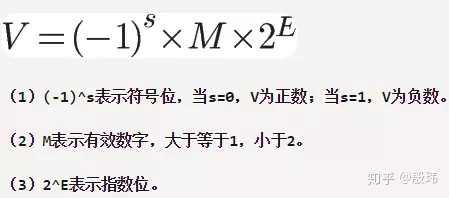
IEEE 754 stipulates that for a 32-bit floating-point number, the highest 1 bit is the sign bit s, followed by 8 bits of exponent E, and the remaining 23 bits are significant digits M.

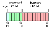
Half-precision floating-point storage-FP16 occupies 2 bytes, a total of 16 bits, of which 1 bit is the sign bit (0 is positive, 1 is negative), 5 bits are the exponent bits, and 10 bits are the mantissa bits.
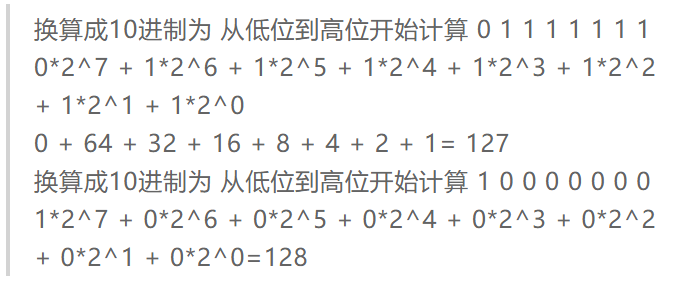
Integer storage-INT8, an eight-bit integer, occupies 1 byte, a total of 8 bits, of which 1 bit is the sign bit (0 is positive, 1 is negative), and 7 are the data bits.
Integer calculations are easy to understand and are made up of 2 raised to the 7th power within the range of (-128-127).
Concept of operating conditions (operating frequency)Both GPU and CPU have working frequencies, the higher the frequency, the higher the performance, but at the same time, their power consumption and heat generation will be higher. In general, overclocking means changing the operating frequency to improve performance. The Xavier (GPU) has a power consumption of 20W, a single-precision floating-point performance of 1.3TFLOPS, and a Tensor core performance of 20 TOPS. After unlocking to 30W, it can reach 30 TOPS. The reason for the term TOPS per watt is to avoid the problem of overclocking. In addition, the power consumption here often refers to the power consumption and computing power ratio of the unit chip itself, without considering DRAM. In deep learning computing, data is frequently accessed, and in extreme cases, power consumption may not be lower than that of the computing unit.
The actual operating frequency may not be the same as the set working frequency, which often depends on temperature and voltage. In the design of integrated circuits, simulation or EDA will provide three common state analyses.
-
WCS (Worst Case Slow): slow process, high temperature, lowest voltage.
-
TYP (typical): typical process, nominal temperature, nominal voltage.
-
BCF (Best Case Fast): fast process, lowest temperature, high voltage.
Assuming a chip with an operating frequency of 2 GHz, a typical temperature of 25°C, and a voltage of 0.8V, its computing power is 2 TOPS. Under WCS, with a temperature of 125 degrees and a voltage of 0.72V, the frequency will drop to 1 GHz and the computing power will drop to 1 TOPS. The TOPS often advertised are the results under BCF.
Calculation method of theoretical TOPS
The TOPS often advertised are the theoretical values of the computing unit, rather than the actual values of the entire hardware system. The actual values depend more on the internal SRAM, external DRAM, instruction set, and model optimization degree. In the worst case, the actual value may be only 1/10 of the theoretical value or even lower, generally only 50% of utilization.
The theoretical value depends on the operating precision, the number of MACs, and operating frequency. It can be roughly simplified as the number of MACs under INT8 precision is equivalent to half of that under FP16 precision. Further, under FP32, it is halved again, and so on.Assuming there are 512 MAC computation units with a frequency of 1GHz and the data structure and precision of INT8, the computational power is 512 x 2 x 1 GHz = 1000 Billion Operations/Second = 1 TOPS (Tera-Operations/second). For FP16 precision, the computational power would be 0.5 TOPS, and for FP32 precision, it would be 0.25TOPS. The NVIDIA Tesla V100 has 640 Tensor cores, each with 64 MAC computation units, and a frequency of approximately 1.480GHz. Therefore, the computational power under INT8 would be 640 x 64 x 2 x 1.480 GHz=121TOPS.
The gap between actual and theoretical TOPS is significant – matching remains the core issue
ResNet-50 requires approximately 7 billion MAC operations per second, and the NVIDIA Tesla T4 can process 3,920 images of size 224 * 224 per second, which equates to 27,440 Billion Operations/second = 27.4 TrillionOperations/Second = 27.4 TOPS. The theoretical computational power of the NVIDIA Tesla T4 is 130 TOPS, but in reality, it only has 27.4 TOPS.
The main factor determining the actual computational power is the bandwidth of the memory (SRAM and DRAM). The theoretical computational power of Google’s first-generation TPU is 90 TOPS, but the worst actual computational power is only 1/9, or 10 TOPS, because the bandwidth of the first-generation memory is only 34GB/s. In contrast, the second-generation TPU uses HBM memory, increasing the bandwidth to 600GB/s (the total memory bandwidth of a single-chip TPU V2 board is 2400GB/s). This discussion is still about a static issue, and the first-generation TPU was primarily designed for mainstream algorithms, with poor matching between its computational power and memory.
Even if the matching between memory and computational power is done well for mainstream algorithms, the situation will not improve significantly from a dynamic perspective because, regardless of the algorithms used, it remains difficult to match the memory and computational power effectively.The algorithm commonly uses “operational intensity” or “arithmetic intensity” to represent the demand for memory bandwidth, measured in OPs/byte. This indicates the number of operations that can be performed per unit data input on average. The higher the operational intensity, the more operations can be supported per unit data input, indicating a lower demand for memory bandwidth.
Let’s use an example for illustration. For a 3×3 convolution operation with a stride of 1, assuming the input feature plane size is 64×64 and both input and output features are equal to 1. It requires a total of 62×62 convolution operations, each requiring 3×3=9 multiplications and additions, resulting in a total of 34,596 calculations. The amount of data required (assuming both data and convolutional kernels use single-precision floating-point, 2bytes) is 64x64x2 (input data) + 3x3x2 (convolution kernel data) = 8,210 bytes. Therefore, the operational intensity is 34,596/8,210 = 4.21. If we switch to a 1×1 convolution, the total number of calculations becomes 64×64 = 4,096, and the amount of data required is 64x64x2 + 1x1x2 = 8,194. Obviously, switching to 1×1 convolution can reduce the amount of computation by nearly 9 times, but the operational intensity also drops to 0.5, indicating a nearly 9-fold increase in memory bandwidth demand. Therefore, if the memory bandwidth cannot meet the computation requirements for 1×1 convolution, although switching to a 1×1 convolution can reduce the amount of calculation by nearly 9 times, it cannot improve the calculation speed by 9 times.Deep learning computing devices have two bottlenecks: processor computing power and compute bandwidth. To analyze which one limits the computing performance, we can use the Roofline model, which plots compute performance (y-axis) against algorithmic compute intensity (x-axis). The Roofline curve is divided into two parts: the ascending region on the left and the saturation region on the right. When the algorithmic compute intensity is low, the curve is in the ascending region, indicating that the computing performance is actually limited by memory bandwidth, and many computing processing units are idle. As the algorithmic compute intensity increases, i.e., more computations can be performed on the same amount of data, the number of idle processing units decreases, and computing performance increases. Then, as the compute intensity becomes even higher, the number of idle processing units continues to decrease until all processing units are in use. At this point, the Roofline curve enters the saturation region, where there are no more processing units available for use, regardless of how high the compute intensity is. This is the point where computing performance no longer improves, or where computing performance encounters a “roof” determined by the computing capability (rather than the memory bandwidth).
Using the example of 3×3 and 1×1 convolutions, the 3×3 convolution may be in the saturation region on the right side of the Roofline curve, while the 1×1 convolution may be in the ascending region on the left side of the curve due to its lower compute intensity. As a result, the computing performance of the 1×1 convolution may decrease and fail to reach peak performance. Although the computational complexity of the 1×1 convolution decreases by almost 9 times, the actual computing time is not one-ninth that of the 3×3 convolution due to the decreased computing performance.
Most AI algorithm companies want to customize or develop their own computing platforms because the performance of algorithms is often closely tied to hardware design. Pursuing modularity often sacrifices utilization rates, so improving utilization rates requires integrated software and hardware design. The design of the chip depends on whether your algorithm is best suited for GPU or CPU, how much memory is required when using multiple MACs at the same time, etc. Alternatively, given a chip, how can my algorithm be compatible? Should I reduce the number of memory accesses to increase utilization rates, or should I migrate some rule-based algorithms from CPU to GPU-based deep learning implementations? Integrated consideration of software and hardware is often necessary to fully utilize system performance.
This article is a translation by ChatGPT of a Chinese report from 42HOW. If you have any questions about it, please email bd@42how.com.