Lidar, also known as Light Detection and Ranging, is an abbreviated term for laser detection and ranging systems. It analyzes the reflection energy size on the surface of a target object, the amplitude, frequency, and phase of the reflected spectrum by measuring the propagation distance between the sensor emitter and the target object. In this way, it presents the accurate 3D structural information of the target object.
Lidar has been widely developed since the invention of lasers in the 1960s. Currently, lidar manufacturers mainly use laser emitters with wavelengths of 905nm and 1550nm. The use of 1550nm wavelength lasers means that the power of lidar using them can be quite high without causing retinal damage as the light is not easily transmitted in human eye liquid. Higher power means greater detection distance, and longer wavelengths mean easier penetration of dust and haze. However, due to cost reasons, the production of lidar with a wavelength of 1550nm requires the use of expensive gallium arsenide materials. Manufacturers mostly opt for using silicon materials to produce lidar that is close to the visible light wavelength of 905nm and strictly limit the power of the emitter, to avoid causing permanent eye damage.
Currently, the main principle of measuring distance is the time-of-flight method, which calculates the distance to the target object by using the time interval between the pulse signal emitted by the transmitter and the reflected pulse signal received by the receiver.
There is also the coherent method, which is the FMCW (Frequency Modulated Continuous Wave) lidar. The FMCW lidar emits a continuous beam of light with the frequency stably changing over time. As the frequency of the light source is constantly changing, differences in the transmission distance of the beam of light will cause differences in frequency. After the echo signal is mixed with the local oscillator signal and filtered by a low-pass filter, the resulting difference frequency signal is a function of the beam of light’s round-trip time. The FMCW lidar does not suffer from interference from other lidars or sunlight, has no blind range, and can also measure the velocity and distance of objects using the Doppler frequency shift. The FMCW lidar concept is not new, but it faces many technical challenges, such as linewidth limitations for laser emission, frequency range of linearly modulated pulses, linearity of linear pulse frequency changes, and the repeatability of individual linearly modulated pulses.
The AMCW (Amplitude Modulated Continuous Wave) lidar is similar to the basic time-of-flight system used in that it emits a signal and measures the time it takes for the laser to reflect back. However, the difference is that the time-of-flight system only emits one pulse, while AMCW lidar adjusts the strength of the emitted light by changing the polarity current in the laser diode to achieve modulation.
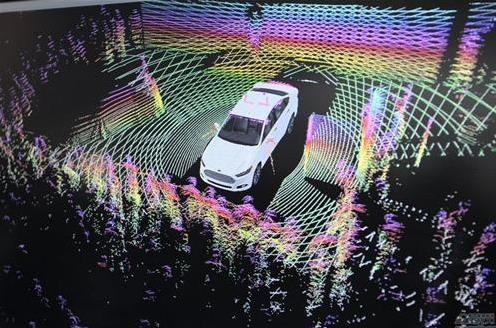
Lidar is primarily used for measuring distance, positioning, and 3D representation of surface objects. As an important sensor, it is widely used in the field of autonomous driving and unmanned aerial vehicles.
The Structure of LiDARThe main components of a LiDAR system include laser emission, reception, scanner, lens antenna and signal processing circuits. There are two main types of laser emission: one is laser diode, usually made of silicon and gallium arsenide substrates, and the other is the currently popular vertical-cavity surface-emitting laser (VCSEL) (such as LiDAR on the iPhone). The advantage of VCSEL is that it is low-cost, small in size, and low in power consumption. The disadvantage is that its effective distance is relatively short and requires multiple amplifications to achieve the effective distance for cars.
LiDAR sensors mainly use the principle of laser ranging. The appropriate structure is manufactured to enable the device to emit laser beams in multiple directions and to measure the round-trip time of the laser, thus distinguishing the different structures of LiDAR.
Mechanical Type
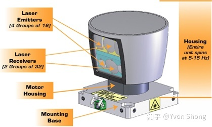
Taking Velodyne’s 2007 LiDAR as an example, it stacks 64 laser diodes vertically together and rotates the entire unit many times per second. The emission system and reception system have a physical meaning of rotation. By continuously rotating the emitter, the laser spot is turned into a line, and multiple beam emitters are arranged vertically to form a surface for 3D scanning and information reception. However, due to the complex mechanical structure required to achieve high-frequency and accurate rotation, the average failure time is only 1000-3000 hours, which makes it difficult to meet the minimum requirement of 13,000 hours for car manufacturers.
Solid-state Type (MEMS)
The solid-state LiDAR utilizes the technology of micro-electromechanical systems to drive the rotating mirror and reflect the laser beam in different directions. The advantages of solid-state LiDAR include fast data acquisition speed, high resolution, and strong adaptability to temperature and vibration. By controlling the beam, the detection points (point cloud) can be distributed arbitrarily, for example, mainly scanning the distant front on the highway, strengthening the side scanning at the intersection, and not completely ignoring it.
Optical Phased Array Type (OPA)
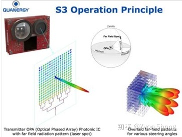
The phased array emitter is composed of several emission and reception units in an array. By changing the voltage loaded on different units, the light wave characteristics of different units are changed, and the light waves emitted from each unit can be independently controlled. By adjusting the phase relationship between the light waves radiated from each phase control unit in the set direction, interference that enhances each other is generated, thus realizing a high-intensity beam in the designed direction, while the light waves emitted from various units in other directions interfere with each other. Each phase control unit in the phased array can make one or more high-intensity beams follow the designed direction in the spatial scan under program control.
 However, the manufacturing process of optical phased arrays is challenging due to the requirement that the dimension of each array unit cannot exceed half a wavelength. The wavelength of most current LiDAR tasks is around 1 micron, which means that the dimension of each array unit must be no larger than 500 nanometers. Moreover, the more arrays there are, the smaller the size of each array unit, and the more the energy concentrates towards the main lobe, which demands higher precision in processing. Additionally, the selection of materials is also a crucial factor.
FLASH (Full-field LiDAR Arrays for Solid-state High-resolution LiDAR)
FLASH is currently the most mainstream technology among all solid-state LiDARs, with its principle based on flash LiDAR technology. As opposed to MEMS or OPA schemes that require scanning, FLASH emits laser in a short time directly to cover the detection area, and utilizes highly sensitive receivers to establish a depiction of the surroundings.
Hardware Parameters
We will take the best-performing MEMS LiDAR as an example to illustrate the key hardware parameters.
Field of View and Resolution
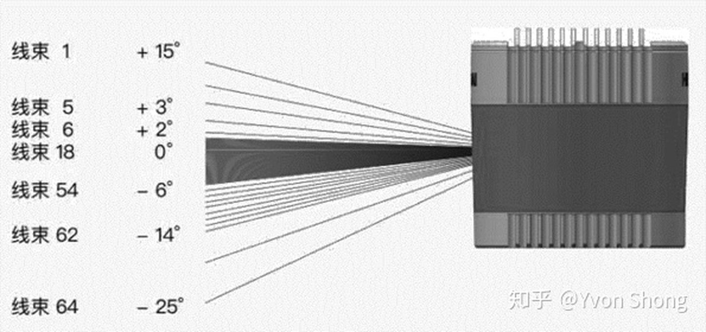
The field of view of a LiDAR can be divided into horizontal and vertical fields of view. The horizontal field of view denoting the angle range that can be observed in a horizontal direction is 360° for a spinning LiDAR that rotates once. The vertical field of view indicates the angle that can be observed in a vertical direction and is generally 40°. However, the field of view is not distributed symmetrically and uniformly because we mainly need to scan obstacles on the road instead of directing lasers towards the sky. To make better use of the lasers, the laser beam will tilt downwards by a certain angle, and to detect the obstacles while also concentrating the laser beam on the central part of interest, the laser beam is not evenly distributed vertically, with greater density in the middle and sparser at the sides. The figure below shows the beam distribution of the Velodyne 64-line LiDAR, which includes a certain offset, with upward angle at 15° and downward angle at 25°, and with denser laser beams in the middle and sparser on both sides.
Echo Mode
Since the LiDAR receiver is receiving lasers emitted by the transmitter, there may be a situation where the same transmitter passes through multiple objects, and the corresponding receiver receives multiple echoes. The echo mode is used to adjust the content contained in the output data packet. In single echo mode, each data block includes ranging data of 64 laser channels, which can be selected as the strongest or the last echo. In dual echo mode, each pair of data blocks corresponds to the different echo ranging data of 64 lasers emitted during the same round, such as the strongest echo and the latest echo.
Point FrequencyThe number of collected points per cycle depends on the scan frequency and the horizontal resolution, which is also known as the number of points scanned horizontally. For example, if the horizontal resolution of a LiDAR is 0.2°, then it will scan 1800 times horizontally, which means it will scan 115200 points per scanning cycle for a 64-line LiDAR such as Velodyne. The scanning frequency also affects the number of points collected per cycle – the faster the scanning speed, the fewer the points collected.
The effective detection distance of a LiDAR varies with the distance being measured. Since the laser emitter and receiver cannot be located in the same position, there is a small amount of error present in the optics system of the LiDAR, which is more pronounced in the TOF (time of flight) LiDAR. The measurement accuracy depends on the accuracy of the system clock, and this accuracy decreases over time due to accumulated errors. Moreover, as the distance being measured increases, the received signal becomes weaker, which affects the receiver’s ability to locate the peak time and, consequently, the accuracy of measurements. Additionally, the effective detection distance of the LiDAR is related to the minimum vertical resolution and angle resolution. If the angle between two laser beams is 0.4°, then at a detection distance of 200m, the distance between the two laser beams is approximately 1.4m. This means that beyond 200m, the LiDAR can only detect obstacles that are higher than 1.4m. Furthermore, the number of points that need to be sampled for obstacle recognition increases with distance, and the sampling rate decreases with distance. Therefore, it is more difficult to identify the precise types of obstacles as the distance increases.
Data from LiDAR
3D PointsFor a rotating LiDAR, the obtained three-dimensional points are observations of multiple points in a polar coordinate system, including the vertical and horizontal angle of the laser emitter and the distance obtained through the calculation of the laser echo time. However, LiDAR usually outputs observations in a Cartesian coordinate system. The first reason is that LiDAR has high efficiency in measuring in a polar coordinate system, but this is only for rotating LiDAR. There are also many array LiDARs currently available. Secondly, the Cartesian coordinate system is more intuitive. Projection, rotation, and translation are more concise. The calculation of features such as normal vectors, curvatures, vertices, and other features has a smaller computational load, and the indexing and search of point clouds are more efficient.
For MEMS-based LiDARs, the sampling period is one polarization mirror rotation period. Under a sampling frequency of 10 Hz, the sampling period is 0.1 seconds. However, due to the high-speed movement of the carrier itself, we need to eliminate motion distortion to compensate for the motion during the sampling period.
Reflection Intensity
In each LiDAR return, in addition to the reflection intensity calculated based on velocity and time, it actually refers to the ratio of the laser echo power to the emission power. The reflection intensity of the laser can be well characterized by the following model based on the existing optical model.
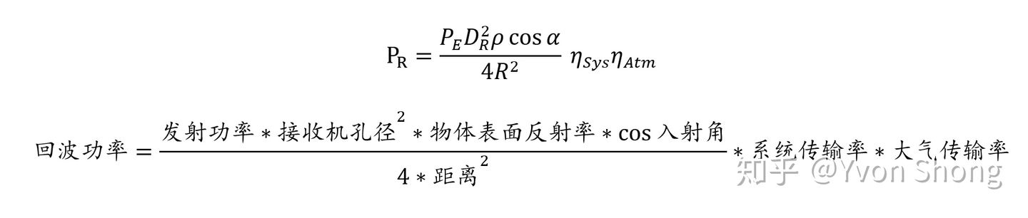
We can see that the reflection rate of the laser point is inversely proportional to the distance squared and inversely proportional to the incident angle. The incident angle is the angle between the incident light and the surface normal of the object.
Timestamp and Encoding Information
LiDAR usually supports hardware-level timing, that is, the LiDAR data can be triggered by hardware trigger and assigned a timestamp for each frame of data. Usually, there are three types of time synchronization interfaces supported: 1. IEEE 15882008 synchronization, which follows the Precision Time Protocol and achieves accurate clock synchronization through Ethernet for measuring and system control. 2. Pulse synchronization (PPS), the pulse synchronization implements data synchronization through the synchronization signal line. 3. GPS synchronization (PPS+UTC), which realizes data synchronization through the synchronization signal line and UTC time (GPS time).
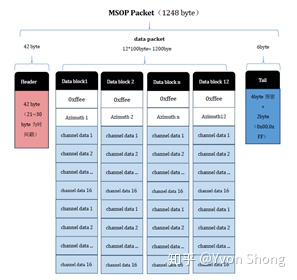
Then we obtain a string of data packets from the LiDAR hardware, and we need to drive it once to parse it into a format commonly used for point clouds, such as ROSMSG or PCL point cloud format. Taking the data of the most common rotating LiDAR as an example, the data is 10 Hz, which means that the LiDAR rotates one circle in 0.1s and slices the hardware-obtained data into different packets according to different angles. The following is a schematic diagram of a packet data package definition.
Diagram of a LiDAR data packet definition.The packets contain data of all points in the current sector, including timestamps, xyz data, emission intensity of each point, and the id of the laser emitter that the point comes from.
Newer LiDARs, such as the Livox Horizon LiDAR, also include multi-echo information and noise information, with the following format:
Each marker information consists of a byte: bits 7 and 6 are the first group, bits 5 and 4 are the second group, bits 3 and 2 are the third group, and bits 1 and 0 are the fourth group.
The second group represents the echo sequence of the sampling point. As Livox Horizon uses coaxial optics, even if there is no external object to be measured, its internal optical system will still produce an echo, which is recorded as the 0th echo. Subsequently, if there are detectable objects in the laser emission direction, the first echo returned to the system is recorded as the 1st echo, followed by the 2nd echo, and so on. If the detected object is too close (e.g., 1.5m), the 1st echo will be merged into the 0th echo, which is recorded as the 0th echo.
The third group determines whether the sampling point is a noise point based on the energy strength of the echo. Typically, the energy of echoes caused by interference such as dust, rain, and snow is very small. Currently, the confidence level of noise points is divided into two categories according to the energy strength of the echo: 01 indicates that the echo energy is weak and the sampling point is likely a noise point, such as dust particles; 10 indicates that the echo energy is moderate and the sampling point is moderately likely a noise point, such as rain and fog noise. The lower the confidence level of the noise point, the lower the likelihood of it being a noise point.
The fourth group determines whether the sampling point is a noise point based on its spatial location. For example, when the ranging of laser detection is only in two distances that are very close to each other, filamentous noise may occur between the two objects. Currently, different confidence levels of noise points are divided into three categories. The lower the confidence level of the noise point, the lower the likelihood of it being a noise point.
The Role of LiDAR
Perception
We can use LiDAR to depict the sparse three-dimensional world and cluster the denser obstacle point cloud, enabling obstacle perception. With the breakthrough in detection and segmentation technology brought about by deep learning, LiDAR can efficiently detect pedestrians and vehicles, outputting detection boxes or labels for each point in the point cloud. Some researchers even attempt to use LiDAR to detect lane markings on the ground.In the field of three-dimensional object recognition, the initial research mainly focused on simple shapes such as cubes, cylinders, cones, and quadric surfaces. However, these shapes have limited capability to express real-world objects, and the vast majority of targets are difficult to approximate using these shapes or their combinations. Subsequent research has mainly focused on the recognition of three-dimensional free-form objects, which are objects with well-defined continuous normal vectors throughout the surface, except for vertices, edges, and sharp corners (such as aircraft, cars, ships, buildings, sculptures, and terrain). As most objects in the real world can be considered as free-form objects, the research on 3D free-form object recognition algorithms has greatly expanded the scope of the recognition system. In the past two decades, the amount of data targeted for 3D object recognition tasks has been increasing, the difficulty of recognition has been increasing, and the recognition rate has also been continuously improving. However, how to achieve detection, recognition, and segmentation of the interested targets in complex scenes that contain occlusion, background interference, noise, outliers, and changes in data resolution, still remains a challenging problem.
Registration
In three-dimensional model reconstruction, the initial research focused on point cloud fine registration, point cloud fusion, and 3D surface reconstruction when both adjacency relationships and initial poses are known. Here, adjacency relationship is used to indicate which point clouds have a certain overlap with a given point cloud, and this relationship is usually obtained by recording the scanning order of each point cloud. The initial pose depends on turntable calibration, object surface marker points, or manually selecting corresponding points. Such algorithms require a lot of manual intervention and therefore have a low degree of automation. Subsequently, researchers turned to three-dimensional model reconstruction when the adjacency relationship between the point clouds is known, but the initial pose is unknown. Common methods include key point matching, line matching, and face matching algorithms. In practical applications, often times the adjacency relationships between point clouds are unknown. To address this, researchers developed minimum spanning tree algorithms and connection graph algorithms to calculate the adjacency relationships. Overall, the development trend of 3D model reconstruction algorithms is towards higher automation, less manual intervention, and broader applications. However, existing algorithms still have issues such as high computational complexity, can only deal with single objects, and are sensitive to background interference. The main challenge is developing a fully automatic 3D model reconstruction algorithm that has low computational complexity and does not depend on prior knowledge.Given two sets of three-dimensional data points from different coordinate systems, find the transformation relationship between the two sets of points to unify them into the same coordinate system. This process is called registration. The goal of registration is to find the relative position and orientation of separately acquired views in a global coordinate framework so that their intersecting regions completely overlap. For each set of point cloud data obtained from different views, the point cloud data is likely to be completely different and requires a single point cloud model that can align them together for subsequent processing steps such as segmentation and model reconstruction. Currently, the most common algorithms for registration are ICP and its variants, NDT algorithm, and feature-based matching.
The ICP algorithm was first proposed by Chen and Medioni, and Besl and McKay. Essentially, the algorithm is an optimal registration method based on least squares. The algorithm repeatedly selects corresponding point pairs and calculates the optimal rigid transformation until the loss function defined by the Euclidean distance of the point pairs satisfies the convergence accuracy requirements for correct registration. The main purpose of the widely used ICP algorithm is to find the rotation and translation parameters to align two point clouds in different coordinate systems using one of them as the global coordinate system and the other after rotation and translation to overlap completely with the overlapping part of the two point clouds.
The basic idea of the NDT algorithm is to construct the multidimensional normal distribution based on the reference data, if the transformation parameters can make the matching between two laser data sets very good, then the probability density of the transformed points in the reference system will be very large. Then, an optimization method is used to find the transformation parameters that make the sum of probability densities maximum, at which point the two laser point cloud data will match the best. This leads to the transformation relationship.
Local feature extraction typically includes two steps of key point detection and local feature description, which form the foundation and key for 3D model reconstruction and object recognition. In the field of 2D images, algorithms based on local features have achieved a lot of results in the past decade and have been successfully applied in image retrieval, object recognition, panorama stitching, unmanned system navigation, and image data mining. Similarly, local feature extraction of point clouds has also made some progress in recent years.
When the three-dimensional points are relatively dense, features and their descriptors can be extracted similar to vision, mainly by selecting points with distinguishing geometric attributes (such as normals and curvatures) and computing their descriptors based on the geometric attributes of their local neighborhood. However, when processing single-frame point cloud data obtained from the laser scanner currently available on the market, point clouds are relatively sparse, and feature points are mainly obtained based on the curvature of the ring obtained by each laser scanner during scanning.
Odometry and LocalizationAfter obtaining the relative pose transformation relationship based on registration between two point cloud data, we can use the data obtained from LiDAR sensors to estimate the relationship between the pose changes of the carrier object and time. For example, we can match the current frame with the previous frame data or match it with the accumulated stacked sub-map to obtain the pose transformation relationship and achieve the function of odometer.
When we match the current frame with the entire point cloud map, we can obtain the pose of the sensor in the entire map and achieve positioning in the map.
Trends of LiDAR
Sensor standardization
Solid-state LiDAR eliminates mechanical structures and solves current problems with cost and reliability of mechanical rotating LiDAR. In addition to these two pain points, the LiDARs currently in mass production have insufficient detection distance and can only meet low-speed scenarios (such as factories, campus, etc.). Daily driving and high-speed driving scenarios are still in the testing phase.
Currently, mechanical LiDARs are extremely expensive. Velodyne’s officially priced 64/32/16-line products are $80,000/$40,000/$8,000 respectively. On the one hand, mechanical LiDAR consists of precise components such as light sources, mirrors, receivers, microcontroller motors, etc., making it difficult to manufacture and costly. On the other hand, LiDARs have not yet entered mass-produced vehicles, and demand is low, so fixed expenses such as research and development costs cannot be amortized. After producing one million units of VLP-32, its price will drop to around $400.
Multi-sensor fusion
Among environmental monitoring sensors, ultrasonic radar is mainly used for close-range obstacle detection in reversing radar and automatic parking. Cameras, millimeter-wave radar, and LiDAR are widely used in various ADAS functions. The detection parameters of these four types of sensors differ in detection distance, resolution, and angular resolution, corresponding to the strengths and weaknesses of object detection capability, recognition classification capability, 3D modeling, and resistance to harsh weather conditions. Various sensors can form a good complementary advantage, and the fusion of sensors has become a mainstream choice.
This article is a translation by ChatGPT of a Chinese report from 42HOW. If you have any questions about it, please email bd@42how.com.