Introduction
In the previous two issues of “Introduction to Autonomous Driving Technology,” I illustrated some basic algorithms in the field of computer vision using lane detection as an example. By applying image processing algorithms and debugging algorithm thresholds, detecting and tracking lane lines can be achieved.
The lane detection and tracking project is mainly accomplished by setting ROI (region of interest) and debugging algorithm thresholds in a rule-based manner to realize lane detection. With the development of artificial intelligence technology, deep learning has been increasingly used for object recognition in the field of image processing in recent years. Using deep learning to recognize images not only improves performance robustness but also achieves higher recognition rates compared with rule-based approaches.
In this sharing session, I will provide an introduction to deep learning related knowledge by taking the traffic sign classification project offered in the Udacity Self-Driving Engineer Nanodegree as an example.
Main Text
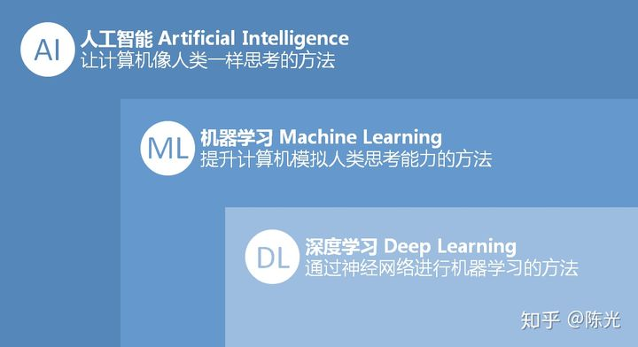
Recognize the relationship between artificial intelligence, machine learning, and deep learning through a simple image. It can be seen that deep learning is a branch of machine learning, and machine learning is a branch of artificial intelligence.
Artificial intelligence can be traced back to the 1950s. Due to the limited computing power at that time, artificial intelligence technology did not develop well. It was not until the 1980s when computer computing power increased significantly that artificial intelligence began to develop vigorously, leading to the emergence of machine learning technology. The appearance of machine learning helped to solve many simple problems such as junk mail classification and housing price estimation, and also assisted in solving complex problems such as image recognition, but the accuracy did not meet expectations. It was not until the emergence of deep learning technology (machine learning through neural networks) and parallel computing technology that the accuracy of complex problems such as image recognition was greatly improved, surpassing the level of human recognition. More and more scientists, engineers, and capital have invested in the field of deep learning.
Artificial intelligence is mainly used to solve two major problems: prediction (regression) and classification. There are many examples of prediction in life, such as predicting the price of a house based on information such as its area, or predicting this year’s sales based on sales in the previous few years. There are also many classification problems such as judging the rise and fall of stocks and recognizing objects (such as handwritten numbers and letters) in images.
Understanding Neural Networks
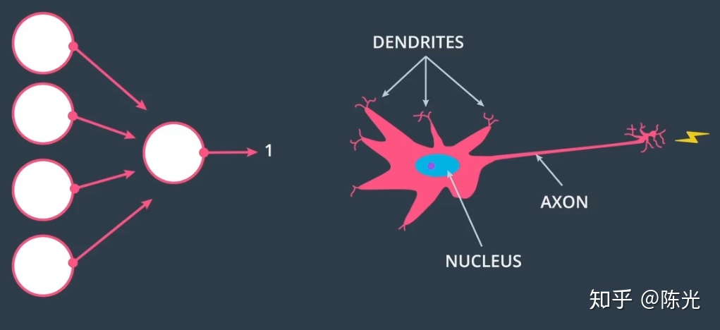
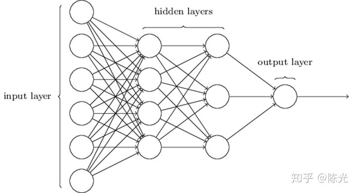
When it comes to neural networks, we always see networks composed of circles and lines as shown below. The reason for drawing this way is explained below.
 Translation:
Human neurons receive data through multiple dendrites and send signals through axons after processing. As a result, the network diagram we built is also called a neural network.
Through an example of calculating house prices, we can explain the circles and lines here.
In an area, the most direct factor affecting a house price is the house area. The larger the area, the higher the price.
That is, house price = house area * price per square meter. We can represent this relationship with two circles and a line:

This is the simplest way to calculate house prices.
However, house prices are also influenced by other factors, such as whether they are renovated or furnished.
Introducing the expenditures on renovation and furniture, we get the formula for house price: house price = house area * price per square meter + renovation area * price per square meter + furniture expenditure * 1. The final housing price composition diagram would look like this:
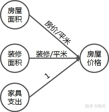
This forms a basic network for predicting house prices. In this network, house area, renovation area, and furniture expenditure are the inputs, house price per square meter and renovation price per square meter are the parameters, and the line segment represents the multiplication operation of these parameters. The house price is the output of this network.
We abstract the above network diagram to make it applicable to more scenarios than just predicting house prices. It looks like this:
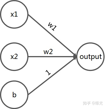
For this simple network, x1, x2, and b are called the inputs of this network. The data in this layer is called the input layer. w1 and w2 are called the parameters of this network. The line segment is the operation rule of the parameter, which can be either arithmetic or complex function. The output of this network is labeled as “output”, and the data in this layer is called the output layer.The house price prediction problem is relatively straightforward and simple, and does not require a complex network to implement. However, when facing complex problems, such as image recognition, it is impossible to describe them clearly using a simple linear network alone. More parameters and more complex calculations (such as sigmoid, relu, etc.) need to be introduced. This is where a network with hidden layers comes in. As the network gets larger, the more parameters it contains, and the network becomes more complex. The more complex the network, the harder it is to explain the role of the parameters in the neural network, which is why deep neural networks are known as “black boxes”.
Neural Network Parameters
Once the house price prediction neural network is built, we can input information such as house area, renovation cost, and furniture expenses into the network to get the price of the house. The more accurate the parameters (house price / square meter, renovation cost / square meter) of the network are, the more accurate the predicted output (house price) will be. Therefore, reasonable parameter settings determine the quality of a neural network.
Before the popularization of deep learning technology, neural network parameters were set based on the developer’s experience. Real data was then input and validated, and the network parameters were continuously adjusted to make the predicted values as close to the real values as possible, thereby obtaining increasingly accurate parameters. This artificial parameter setting method is feasible in shallow neural networks, but becomes impractical when the network parameters reach the thousands or tens of thousands level.
To solve the parameter tuning problem in deep neural networks, experts in the field of deep learning have proposed the theory of backpropagation.
Data is sent from the input layer, goes through a series of calculations in the hidden layer to obtain results, and this process is called forward propagation. The idea of backpropagation is similar to the artificial parameter setting method mentioned earlier, and it also fine-tunes the network by comparing the difference between the predicted values of the network and the real values.
However, the method of backpropagation is different from artificial parameter setting. It requires calculating the predicted value and the real loss function L. The loss function can be understood as the difference between the predicted value and the real value, and the larger the difference, the larger the loss function.After calculating the loss function between the predicted values and the true values, the partial derivatives of the forward propagation parameters with respect to the loss function are computed and passed back to the previous layer of the network. The network parameters are updated using this partial derivative and a coefficient (learning rate) that is multiplied by it. This process is then propagated to the higher layers of the network until all the parameters in the network are updated.
With each set of data, the parameters can be updated using the backpropagation method, which is why deep learning networks become more accurate as the amount of training data increases.
The theory behind backpropagation is extensively covered in Udacity’s Deep Learning Foundation Course for Self-Driving Cars and in the article “Understanding Backpropagation in Neural Networks” which uses a simple network to explain the backpropagation process in a straightforward way.
Training Set, Validation Set, and Test Set
Throughout this discussion, the term “data” has been used to refer to the input to the neural network. In reality, these data have different names in different stages of the neural network. They are the Training Set, Validation Set, and Test Set.
The Training Set and Validation Set are used in the training stage of the neural network model, while the Test Set is used to evaluate the performance of the model after training is complete. To use a simple analogy, the Training Set is like a student’s textbook. The student learns knowledge (trains the model) based on the textbook. The Validation Set is like the homework assignments that the student completes after learning, to help them determine whether they have mastered the content of the textbook. The Test Set is like the final exam, which evaluates the student’s understanding of the material covered in the textbook and homework assignments.
Just as a student’s performance is judged by their final exam results, a neural network model is judged by its performance on the Test Set.
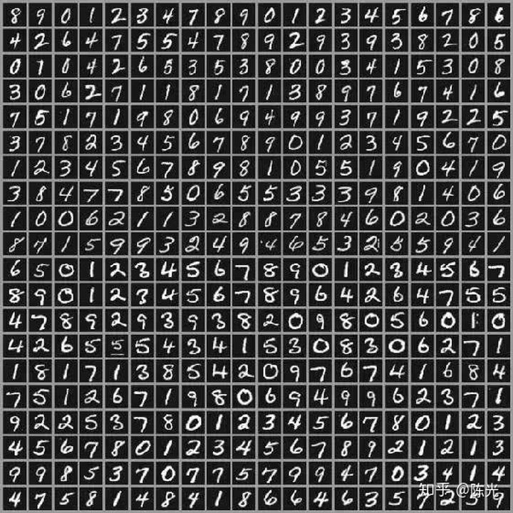
MNIST handwritten digit dataset is one of the most famous datasets in the field of deep learning, consisting of 60,000 training samples and 10,000 test samples. Some of the samples are shown below:
 The following is the English Markdown text that preserves the HTML tags and outputs only the corrections and improvements in a professional manner:
Using the deep learning framework TensorFlow, launched by Google, it is possible to directly obtain the MNIST handwritten digital dataset using the following code:
from tensorflow.examples.tutorials.mnist import input_data

mnist = input_data.read_data_sets ('/home/my_mnist_data',one_hot=True)

train_features = mnist.train.images
test_features = mnist.test.images

train_labels = mnist.train.labels.astype (np.float32)
test_labels = mnist.test.labels.astype (np.float32)
In the code above, train_features and test_features respectively indicate the training set and test set, i.e., the collections of handwritten digital images. train_labels and test_labels are the labels corresponding to the images in the training set and the test set, i.e., the collection of numbers ranging from 0 to 9.
Since the MNIST dataset does not provide a validation set, engineers typically extract 15% to 20% of the data from the training set as the validation set, and the remaining 80% to 85% of the data as the training set to complete the training process.
Using LeNet-5 for Traffic Sign Classification
After having understood the above content, one can have a rough understanding of how neural networks work. By supplementing with some syntax knowledge of TensorFlow, and taking a look at some examples of TensorFlow, one can construct a neural network by oneself.
If faced with complex image processing problems, one needs to use convolutional neural networks (CNNs). CNNs were proposed by the father of convolutional neural networks, Yann Lecun, during his time at the Bell Labs to solve the problem of handwritten digital recognition. Convolution is a special function whose position in the neural network is no different from the four arithmetic operations or some special functions.
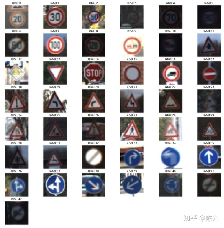
Below, we use the LeNet model proposed by Yann Lecun to train a neural network capable of recognizing traffic signs by importing the training set of traffic signs and applying a convolutional neural network.Firstly, import the data of traffic signs. The Udacity Self-Driving Car Engineer Nanodegree program provides us with a dataset consisting of 34799 training images, 4410 validation images, and 12630 test images belonging to 43 different classes of traffic signs, such as speed limit, turn, and stop signs. Some of the training set samples are shown in the following image:
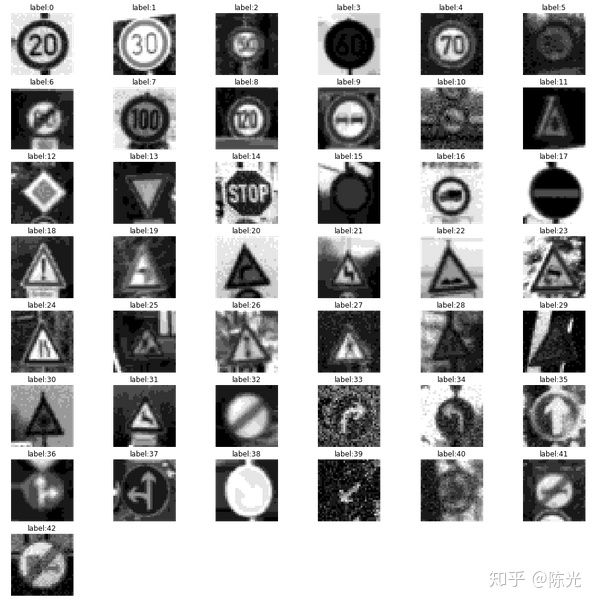
Since LeNet-5 requires input images of size (32 x 32 x 1) with a single channel by default, I preprocessed the training set, validation set, and test set by converting them to grayscale, resizing, and normalizing them. Some of the preprocessed samples are shown below:
LeNet-5 is a relatively simple convolutional neural network, and its structure is shown in the following figure. The input of the network is a two-dimensional image with a single channel, which is processed by two sets of convolutional and pooling layers before passing through fully connected layers and finally using softmax classification as the output layer.
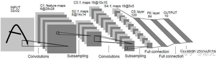
For a more detailed introduction to the LeNet-5 model, please refer to “An Analysis of the LeNet-5”.
There is a problem during training: the accuracy of the training set is high, but the accuracy of the validation set is low. This indicates that the model is overfitting during training, resulting in a recognition rate of only about 89% for the validation set, while the course requirement is to achieve more than 93%.
To solve the problem of low model accuracy caused by overfitting, I did two things:
Use the imgaug library for data augmentation
By using the imgaug library, it is easy to perform data augmentation such as flipping, translating, rotating, scaling, affine transformation, adding noise, modifying color channels, etc. with simple code. This can achieve the goal of enriching the training set. The following image shows the effect of data augmentation performed on the same image using the imgaug library.
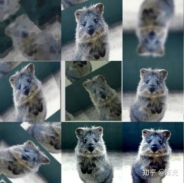
I added random noise, modified the contrast, and flipped horizontally to the training set of traffic signs to perform data augmentation.
Add Dropout function after the fully connected layer in the LeNet-5 model.Adding the Dropout function in the LeNet-5 network allows the network to not rely too much on certain parameters, as these parameters can be dropped at any time. During training, the network is forced to learn all redundant representations to ensure that important information is preserved. When a parameter in the network is dropped, other parameters can still perform the same task, which is the function of Dropout.
Adding the Dropout function to the network can make it more robust and prevent overfitting.
After applying data augmentation and the Dropout function, retraining can make the model achieve an accuracy rate of over 93% in the test set, meeting the requirements.
Conclusion
The above is the complete content of “Traffic Sign Classification: An Introduction to Deep Learning”. Some of the source code, images, and datasets in the article come from Udacity’s Self-Driving Car Engineer Nanodegree Program.
In this sharing, I introduced the theoretical knowledge related to neural networks in deep learning. This includes parameters in neural networks, the principle of backpropagation, and the differences between training, validation, and test sets. Finally, I introduced how to use the LeNet-5 network to implement traffic sign classification and provided solutions to analyze the reasons when the classification effect is not ideal.
In the field of self-driving, deep learning is not only used for object recognition in images, but also widely used in areas such as laser point cloud object classification, trajectory prediction of obstacles, and end-to-end motion control. Mastering the theoretical knowledge and application methods of deep learning can help us solve many difficult problems in the field of self-driving.
Okay (^o^)/~, this sharing comes to an end, see you next time~
This article is a translation by ChatGPT of a Chinese report from 42HOW. If you have any questions about it, please email bd@42how.com.