Introduction
In the “Introduction to Autonomous Driving Technology (Part 18)|Step-by-Step Guide to Implementing Extended Kalman Filtering” and “Introduction to Autonomous Driving Technology (Part 19)| Step-by-Step Guide to Implementing Multi-Sensor Fusion Technology”, I introduced how to use Kalman Filters (KF) and Extended Kalman Filters (EKF) to track obstacles using laser radar and millimeter wave radar data for example. Kalman Filters can solve linear state estimation problems well. When encountering nonlinear state estimation problems, Extended Kalman Filters can linearize nonlinear problems, but there may be some loss of accuracy.
In addition to KF and EKF, there is another classic filtering algorithm called Particle Filter. The idea of the Particle Filter is based on the Monte Carlo method, which uses a set of particles to represent probabilities and can be used in any form of state space model. Compared with other filtering algorithms, Particle Filters have greater advantages in solving nonlinear and non-gaussian problems. In the field of autonomous driving, Particle Filters are often used to solve the localization problem of unmanned vehicles.
This article will explain how Particle Filters solve the localization problem in autonomous driving using the localization course provided by Udacity’s Self-Driving Engineer Degree Program as an example.
The download address of the engineering code and simulation tool provided by Udacity is as follows:
Link: https://pan.baidu.com/s/1HVVvlwgyNmu2AArQ1e7w
Extraction code: kcnk
Body
Before formally introducing the theory of implementing localization through Particle Filters, let’s first understand its working principle intuitively through illustrations.
Map Input
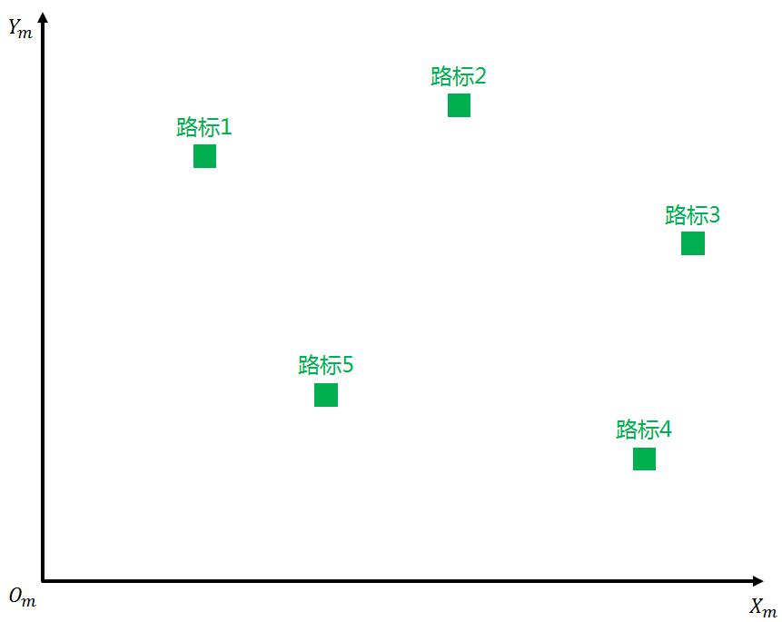
Firstly, we have a local high-precision electronic map with many green landmarks, corresponding to points of interest (POIs) on the high-precision map.
We simplify the current scene into a plane coordinate system, and select a certain reference point Om (m refers to map) as the origin in this coordinate system. The Xm axis points east and the Ym axis points north. In the XmOmYm coordinate system, each landmark has a unique coordinate and ID relative to the origin.
Generally, the position of POIs on a high-precision electronic map is stored in the form of longitude and latitude. By introducing the plane coordinate system, longitude and latitude can be converted into local coordinates. Open source libraries commonly used for coordinate conversion include Geolib and Proj.4. The theory of converting longitude and latitude to local coordinates is not the focus of this article, so we will not elaborate on it here. The following discussions are based on the plane coordinate system.
Initialization
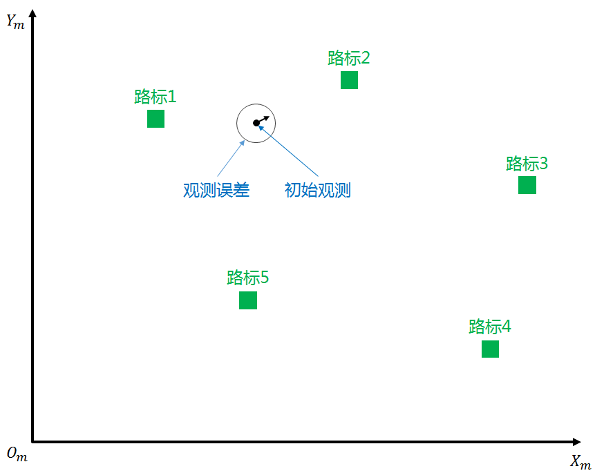 During the initialization of the unmanned vehicle positioning system, it receives the initial GPS observation information, which includes the position XY of the unmanned vehicle in the XmOmYm coordinate system (the position of the black dot in the figure) and the heading angle θ (the angle between the black arrow and the X direction in the figure). Due to measurement errors of the sensors, the true value of the unmanned vehicle position should be near the initial observation position, within the observation error circle shown in the figure.
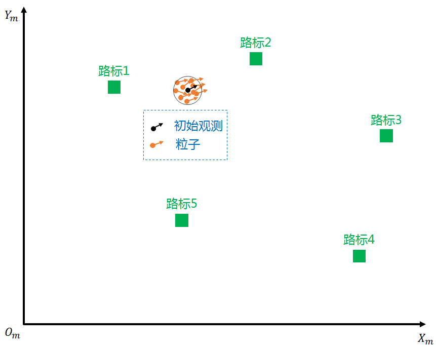
Most sensor measurement errors follow the Gaussian distribution. To create N particles (orange dots) for each position X, Y, and heading angle θ of the initial observation, we add Gaussian noise for each position. When particles are initially created, each particle has an equal weight of 100%. In theory, when N is large enough, there will always be a particle whose position and heading angle is consistent with the true value. If we can find this particle, we can find the true value. This is the basic idea of particle filtering.
Prediction
After initializing all particles based on the GPS position, the unmanned vehicle begins to move. During the movement, the positioning module can receive information such as the vehicle speed v and the change rate of the heading angle yaw_rate, which can be used to estimate the vehicle’s position after a certain time △t.
The process of estimating the vehicle position based on the vehicle speed and the change rate of the heading angle is called odometry. In addition to using vehicle speed and heading angle change rate, other sensors such as IMU can also achieve similar functions.
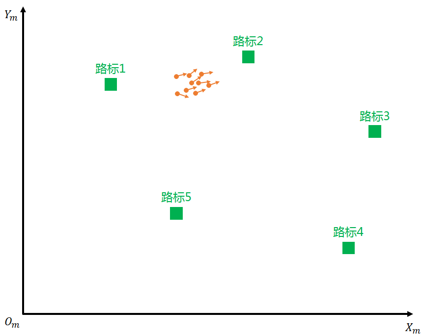
Since each particle could be the true position of the unmanned vehicle, we predict (odometry calculation) for all particles, as shown in the figure below. Each particle has its own initial position and heading angle. After prediction, the distribution of the particle group is no longer so concentrated.
Update Particle Weights
After the particle prediction, we need to update the weights of all particles (the initial weights of all particles are equal). The updating criterion for particle weights is the perception of the unmanned vehicle to the landmark position. Since the vehicle-mounted sensors are installed on the vehicle, the perceived landmark position is based on the vehicle coordinate system.
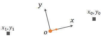
As shown below, (x0,y0) and (x1,y1) are two landmarks detected by the sensor in the vehicle coordinate system.
 We plot the perception results onto a flat coordinate system (which includes the coordinate conversion from the vehicle coordinate system to the flat coordinate system). For readers’ convenience, I only plotted three typical landmarks observed by the particles, as shown below. The green landmarks are on the map, while the observed results of the orange particles are plotted in orange, and those of the purple and blue particles are plotted similarly.
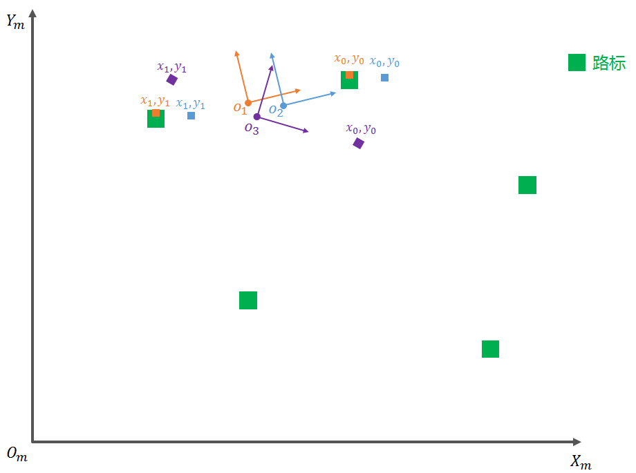
It can be seen intuitively from the figure that among the particles O1, O2, and O3, the sensor’s perceived landmarks that best match the actual landmarks on the map are O1 (orange), followed by O2 (blue), and finally O3 (purple). The lower matching of the blue is due to its position, while the lower matching of the purple is due to its heading.
This also means that after weight update, all particles have the same weight and are updated to weights: particle O1 > particle O2 > particle O3, and particle O1 can be chosen as the current position of the unmanned vehicle. It can be imagined that when the number of particles is large enough, the higher the weight of the particle, the closer its position and heading are to the true value.
Resampling
After updating the weight of each particle using the method mentioned above, we need to delete and add particles, which is called resampling. The purpose of resampling is to delete particles with lower weights while adding new particles around particles with higher weights, while keeping the total number of particles the same.
As the number of resampling increases, the concentration of particles will become higher and higher, and only extremely close to the true value particles will remain. The particle with the highest weight is selected as the position of the unmanned vehicle.
Above, we introduce the application of Particle Filter Algorithm in unmanned vehicle positioning from an intuitive perspective. Below, we will conduct formula derivation and code writing for the particle filter process from a rational perspective.
Code: Map Input
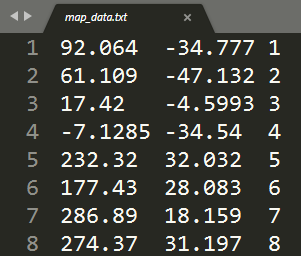
After downloading the project code mentioned earlier, open the data directory and you will see a file named map_data.txt. The file has 42 lines, each representing a landmark (the green blocks in the previous figure), and each landmark has a unique coordinate and ID (starting from 1 and increasing sequentially). The coordinates provided in the map file are not latitude and longitude, but values in meters (i.e., position in a flat coordinate system).
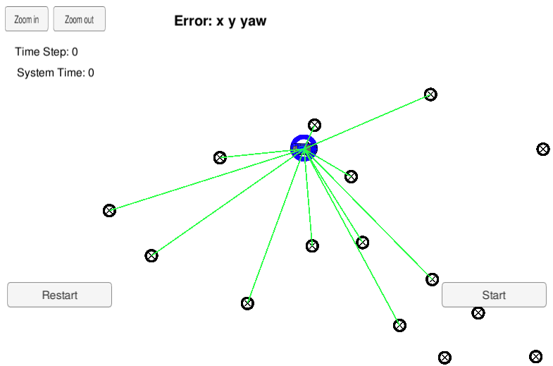
 The road signs are displayed in the simulation as shown in the ⊕ in the figure below. Some road signs have green lines connecting them to the blue car, indicating that these road signs are within the sensing range of the car-mounted sensors and can be detected. The blue car represents the true location (Groundtruth).
Code: Initialization
Particle filter initialization requires an initial position, initial heading, and measurement errors, based on which N particles can be established.
The engineering code establishes a class named ParticleFilter and declares an init function, which requires four parameters as input. The first three are x, y, and theta, which are the initial position and the initial heading, and the fourth parameter is an array that stores measurement errors in the x, y, and heading directions.

Firstly, the number of particles is set to a certain value, such as 100, and then particles are created using a for loop. When a new particle is created, we add a random Gaussian distribution measurement error to the initial position and initial heading. The code for creating new particles is as follows:
void ParticleFilter::init(double x, double y, double theta, double std[]) {
numparticles = 100; // Set the number of particles
particles.resize(numparticles);
std::default_random_engine gen;
std::normal_distribution<double> dist_x(x, std[0]);
std::normal_distribution<double> dist_y(y, std[1]);
std::normal_distribution<double> dist_theta(theta, std[2]);

for (size_t i = 0; i < num_particles; ++i) {```
particles.at(i).x = distx(gen);
particles.at(i).y = disty(gen);
particles.at(i).theta = dist_theta(gen);
particles.at(i).weight = 1.0;
}
is_initialized = true;
}
Code: Prediction
In my previous articles introducing KF and EKF, I discussed obstacle prediction based on the [x,y,x’,y’] model, which simplistically involves only position and velocity but not heading angle estimation. However, in the field of autonomous vehicle localization, heading angle is an important state variable, which necessitates a different model.
A commonly used model in the domain of autonomous vehicle target tracking and state estimation is the CTRV model (Constant Turn Rate and Velocity Magnitude Model).
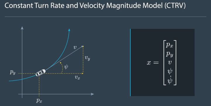
The state equation for the CTRV model is [px, py, v, yaw, yawrate]. Here, px and py denote the lateral and longitudinal coordinates of the vehicle relative to the coordinate system, v represents the speed of the vehicle and its direction is the tangent direction of the travel trajectory (blue line in the figure), yaw represents the vehicle’s heading angle, and yawrate represents the rate of change of the heading angle.
The CTRV model stipulates that within an extremely short time frame (between two observed frames), the speed of the vehicle v and the rate of change of the heading angle yaw_rate remain constant, which means that the vehicle can be assumed to be moving in a circular path between consecutive frames.
The state equation transition from time step k to k+1 is shown below, where △t is the time elapsed between two consecutive time points. For the sake of simplification, yaw is denoted as φ, and yaw_rate is denoted as the derivative of φ.
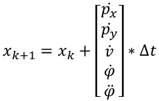
Since the speed of the vehicle v and the rate of change of the heading angle φ’ are constant, the derivative of v and φ” are both zero. This can be used to simplify the equation above using known variables.Translated English Markdown Text:
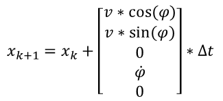
Where △t is the time difference between k and k+1 moments.

Due to the lengthy process of deriving the CTRV model prediction process, which is not the focus of this sharing, I will give the conclusion directly:
- When φ’ is 0, that is, the speed, heading angle change rate, and heading angle do not change, the car travels in a straight line, and only the position changes:

- When φ’ is not 0, the car performs circular motion during the time period between k and k+1, and the state equation changes as follows:
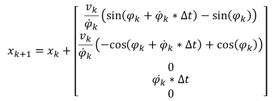
If you are interested in the derivation of the state equation, you can download it via the following link.
Link:https://pan.baidu.com/s/125i9fSsVgGITuo1-8D7vYA
Extracting code:bs5w
The code declares a prediction function, which requires 4 parameters as input. The first parameter, deltat, is the time difference between two consecutive frames, which is △t in the formula; the second parameter, stdpos [], is the prediction noise introduced during prediction; the third parameter, velocity, is the vehicle speed v at moment k, and the fourth parameter is the yawrate at moment k. v and yawrate are the known data observed by the vehicle sensors (speed, heading angle change rate) at moment k.
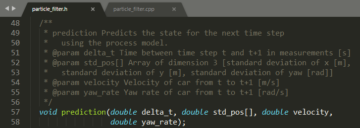
void ParticleFilter:: prediction (double deltat, double stdpos[],
double velocity, double yawrate) {
std::defaultrandomengine gen;“`
std::normaldistribution
std::normaldistribution
std::normaldistribution
for (sizet i = 0; i < numparticles; ++i) {
double x0 = particles.at(i).x;
double y0 = particles.at(i).y;
double theta0 = particles.at(i).theta;
double x_pre = 0.0;
double y_pre = 0.0;
double theta_pre = 0.0;

if (fabs(yaw_rate) < 0.00001) {
    x_pre = x0 + velocity * delta_t * cos(theta0);
    y_pre = y0 + velocity * delta_t * sin(theta0);
    theta_pre = theta0;
} else {
    x_pre = x0 + velocity / yaw_rate * (sin(theta0 + yaw_rate * delta_t) - sin(theta0));
    y_pre = y0 + velocity / yaw_rate * (cos(theta0) - cos(theta0 + yaw_rate * delta_t));
    theta_pre = theta0 + yaw_rate * delta_t;
}
<!-- Unify the angle within 0-2π -->
}
while (theta_pre > 2 * M_PI) theta_pre -= 2. * M_PI;
while (theta_pre < 0.0) theta_pre += 2. * M_PI;
particles.at(i).x = x_pre + noisy_x(gen);
particles.at(i).y = y_pre + noisy_y(gen);
particles.at(i).theta = theta_pre + noisy_theta(gen);
}
```
### Code: Update Particle Weights
Updating the weights of particles from a coding perspective can be divided into the following steps:
1. Transform observed landmarks in the vehicle coordinate system into the map coordinate system.
2. Match the transformed landmarks with landmarks on the map, i.e. data association.
3. Recalculate the particles' weights based on the matching results.
Coordinate Transformation
According to the prediction principle mentioned earlier, we have the position of each particle at time k+1. At the same time, the sensor has observed landmarks in the vehicle coordinate system at time k+1. Therefore, we need to update the weight of each predicted particle. In order to do this, we need to match the observed landmarks with landmarks on the map, i.e., "data association". The key point to this is that all of the landmarks involved in the matching should be in the same coordinate system.
Currently, the reference coordinate system for landmarks on the map is the map coordinate system, and the reference coordinate system for landmarks observed by the sensor on the car is the vehicle coordinate system. Therefore, we need to transform these two coordinate systems into one. As shown in the figure below, we use XmYm to represent the map coordinate system (m for map) and XcYc to represent the vehicle coordinate system (c for car). (xp, yp, θ) represents the position and orientation of the predicted particle in the map coordinate system, and (xc, yc) represents the position of the observed landmark in the vehicle coordinate system.
Now, we need to know how to represent the observed landmark in the map coordinate system.
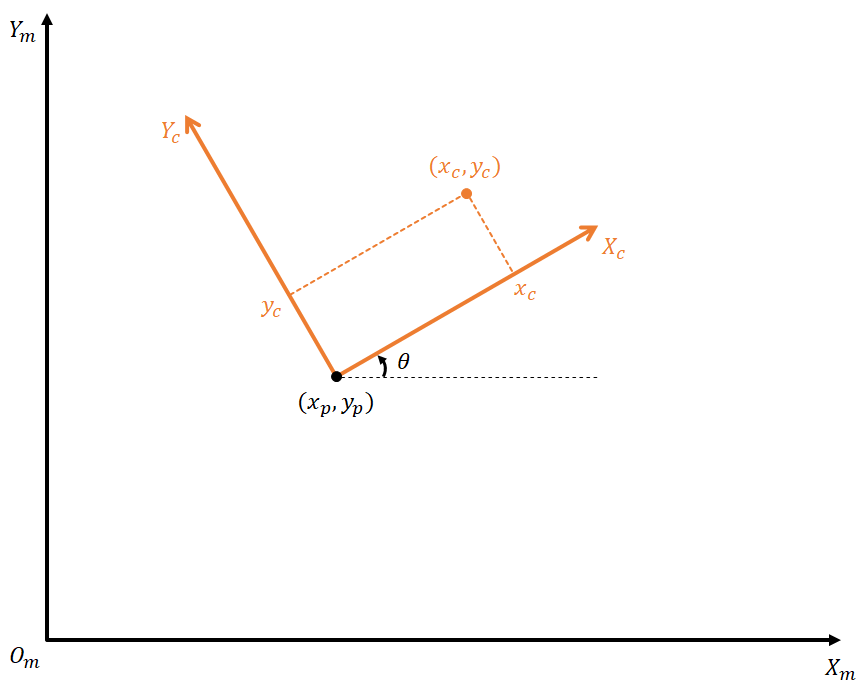
The basic idea of coordinate transformation is to first perform a rotation transformation, and then perform a translation transformation.
First, we ignore the translation and calculate how XmYm can be represented by xc, yc, and θ after rotation. After that, we calculate Ym.Translate the Chinese text in Markdown format below to English in Markdown format, in a professional manner, preserving HTML tags inside Markdown, and only output the corrected and improved parts without explanation:
```
With the origin of the coordinate system in the plane coinciding with the origin of the coordinate system in the car body, auxiliary lines are drawn to determine xm as shown below:

Similarly, with the origin of the coordinate system in the plane coinciding with the origin of the coordinate system in the car body, auxiliary lines are drawn to determine ym as shown below:

The final coordinate transformation relationship can be obtained as follows by adding translation to the rotation transformation calculations:

The following code implemented in C++ is used to transform coordinates, where observations represent all landmarks observed by the unmanned vehicle at time k+1, and obs_in_map is used to store the positions of the observed landmarks in the plane coordinate system after coordinate transformation:

Data Association
After the landmarks observed by the unmanned vehicle are transformed to the plane coordinate system, they will be "associated" with the landmarks on the high-precision map, which means that the corresponding relationship between the observed landmarks and the actual landmarks on the map will be determined.
Landmark association can be considered as a point-to-point association. The simplest and most commonly used association method is called "nearest neighbor", which means finding the nearest point based on distance as the associated point.
The code declares a function called dataAssociation, which takes two parameters as inputs: predicted, which represents the landmarks on the map and each landmark's position x, y in the plane coordinate system, as well as its unique ID, and observations, which represents the observed landmarks after coordinate transformation. After being associated, each observed landmark will be bound to an actual landmark on the map through an ID.
```The implementation of the data association section is not complicated, as shown below. By looping through the data multiple times, we can find the landmark with the smallest distance and assign its ID to the observed landmark, thus establishing an association.
```cpp
void ParticleFilter::dataAssociation(vector<LandmarkObs> predicted, vector<LandmarkObs>& observations) {
for (LandmarkObs& obs : observations) {
double distance_min = std::numeric_limits<double>::max();
for (int i = 0; i < predicted.size (); ++i) {
LandmarkObs pre = predicted [i];
double distance2 = (pre.x - obs.x) * (pre.x - obs.x) + (pre.y - obs.y) * (pre.y - obs.y);
if (distance2 < distance_min) {
distance_min = distance2;
obs.id = pre.id;
}
}
}
}
```
### Calculate Particle Weights
After completing the data association, we will find that each observed landmark has a corresponding landmark in the real world. We can then calculate a weight based on the distance between them, which reflects how well the observed landmark at the current location matches the landmark in the real world.
The formula is as follows:
The code section for calculating particle weights is shown below. First, the true position of the landmark in the real world is obtained by finding the landmark associated with the data ID, and then ux and uy are obtained. After that, the formula is applied to calculate the weight. The weight value will be continuously multiplied by the number of observed landmarks, and the final weight corresponding to each particle is obtained.

### Code: Resampling
After calculating the weight of each particle, the particles with small weights need to be removed and new particles need to be added near the particles with large weights to maintain the same number of particles in the entire particle set.
Resampling can be implemented using the discrete distribution function provided by C++, which is based on the principle of random sampling. First, a discrete distribution set is built based on the weight of each particle, and then a random sample is taken from this set. The larger the weight, the higher the probability of being sampled.
```
void ParticleFilter::resample () {
/**
* Resample particles with replacement with probability proportional
* to their weight.
* You may find std::discrete_distribution helpful here.
* http://en.cppreference.com/w/cpp/numeric/random/discrete_distribution
*/
std::random_device rd;
std::mt19937 gen (rd ());
std::discrete_distribution<> d {std::begin (weights), std::end (weights)};
//build resampled particles
vector<Particle> resampled_particles (num_particles);
markdown
for (size_t i = 0; i < num_particles; ++i) {
    resampled_particles [i] = particles [d (gen)];
}

particles = resampled_particles;

weights.clear ();
After resampling, there are 100 new particles. By repeating the process of prediction, coordinate transformation, data association, and updating weights, the particles will gradually converge and the particle with the highest weight that approaches the true position will be obtained.
Thus, the entire unmanned vehicle positioning function based on particle filtering is completed. The complete project code can be obtained through the following link.
Link: https://pan.baidu.com/s/19UVacwkw5yKEMaD3DR0a4A
Extraction code: glbp
Deploying the above process to run in the project code and turning on the simulator, you can complete the positioning of the unmanned vehicle as shown in the following video. The blue circle that is close to overlapping with the blue car in the video is the position of the unmanned vehicle that we calculated.
Unmanned Vehicle Positioning using Particle Filtering
Conclusion
The above is the process of implementing unmanned vehicle positioning using particle filtering, from intuitive analysis to rational implementation.
Because the main purpose of this article is to introduce the principles and implementation of particle filtering, some simplifications have been made, including high-precision maps, matching algorithms, and other content. In actual unmanned vehicle positioning, positioning elements besides landmarks also include lane lines, traffic signals, and so on, which involves more issues and more complex algorithms.
Alright (^o^)/~, this sharing about particle filtering is completed. If you have any questions, feel free to leave a comment below.
This article is a translation by ChatGPT of a Chinese report from 42HOW. If you have any questions about it, please email bd@42how.com.
