Introduction
In the article “Introduction to autonomous driving technology (13) | Step-by-step teaching you to write a Kalman filter”, I introduced the seven formulas of the Kalman filter (KF) using data from a lidar and implemented the tracking of obstacles of the lidar with C++ code. In the article “Introduction to autonomous driving technology (18) | Step-by-step teaching you to write an extended Kalman filter”, I used data from a millimeter-wave radar to introduce how the extended Kalman filter (EKF) handles nonlinear problems.
Whether it is the Kalman filter processing linear problems or the extended Kalman filter handling nonlinear problems, they only involve tracking obstacles from single sensors. Single sensors have their limitations. For example, the lidar has a more accurate position measurement but cannot measure velocity; the millimeter-wave radar has accurate velocity measurement but is lower in precision for position measurement compared to the lidar. To fully utilize the advantages of various sensors, the technology of multi-sensor fusion has emerged.
Due to multi-sensor fusion being an advanced content for KF and EKF, readers are recommended to read the articles “Introduction to autonomous driving technology (13) | Step-by-step teaching you to write a Kalman filter” and “Introduction to autonomous driving technology (18) | Step-by-step teaching you to write an extended Kalman filter” first to understand the basic theory of the Kalman filter.
This article will use data from a lidar and a millimeter-wave radar detecting the same obstacle to explain the multi-sensor fusion technology. I will provide the multi-sensor data used in the Udacity autonomous driving engineer program and provide code for reading the data to facilitate learning.
The input data for multi-sensor fusion can be obtained through the following link.
Link: https://pan.baidu.com/s/1zU9SgZkMfs75sXt2Odzw Extraction code: umb8
Body
Input data for sensor fusion
After downloading and decompressing the code, you can find a file called sample-laser-radar-measurement-data-2.txt in the data directory, which is the input data for sensor fusion. The scenario for measuring the data is that a lidar and a millimeter-wave radar, which detect obstacles at the same frequency, are fixed at the origin (0,0), and then the two radars trigger alternately to detect the same moving obstacles.
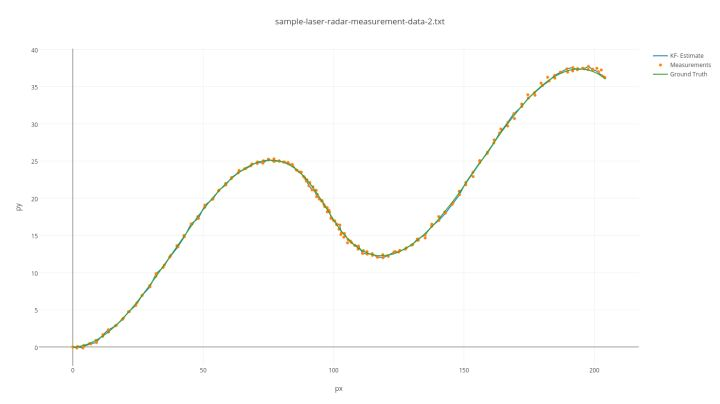
The trajectory of the moving obstacle is shown in the following figure. The green line in the figure is the true motion trajectory (Ground Truth) of the obstacle, and the orange dots represent the detection results of the multi-sensor.
 # Translation
The sensors in the system, namely the Lidar and Radar, trigger detection alternately, resulting in alternating sensor data. In addition to providing measurement values of the sensors, the data also provides ground truth information about the location and velocity of obstacles. This ground truth information can be used to evaluate the performance of the fusion algorithm.
The first letter of each frame indicates which sensor the data comes from. “L” stands for Lidar and “R” stands for Radar.
Lidar can only measure position. The data following the letter L consists of the measured values of the obstacle’s position in the X and Y directions (in meters), the time stamp of the measurement (in microseconds), and the ground truth position and velocity of the obstacle in the X and Y directions (in meters and meters per second, respectively).
Radar can measure the radial distance, angle, and speed of the obstacles. The data following the letter R consists of the distance of the obstacle in the polar coordinate system, the angle (in radians), the mirror velocity (in meters per second), the time stamp of the measurement (in microseconds), and the ground truth position and velocity of the obstacle in the X and Y directions (in meters and meters per second, respectively).
The input data is parsed according to the above rules, similar to the driver layer in autonomous driving technology. The sample-laser-radar-measurement-data-2.txt file is like sensor data sent over a CAN or Ethernet bus network, and the parsing rules are like the protocols used to parse CAN or network data.
In the program, I read the sample-laser-radar-measurement-data-2.txt file and parse each line of data according to the “protocol”. The measured values are stored in the MeasurementPackage structure, and the ground truth values are stored in the GroundTruthPackage structure. Then I iterate through the data using a loop and input them frame by frame into the algorithm. Please refer to the main.cpp function for the specific code.
The internal structure of the MeasurementPackage is shown below:
“` //@ filename: /interface/measurement_package.h
ifndef MEASUREMENTPACKAGEH_
define MEASUREMENTPACKAGEH_
#include "Eigen/Dense"
class MeasurementPackage {
public:
long long timestamp_;
enum SensorType {
LASER,
RADAR
} sensor_type_;
Eigen::VectorXd raw_measurements_;
};
#endif /* MEASUREMENT_PACKAGE_H_ */
The internal structure of GroundTruthPackage is shown below:
//@ filename: /interface/ground_truth_package.h
#ifndef GROUND_TRUTH_PACKAGE_H_
#define GROUND_TRUTH_PACKAGE_H_
#include "Eigen/Dense"
class GroundTruthPackage {
public:
long timestamp_;
enum SensorType {
LASER,
RADAR
} sensor_type_;
Eigen::VectorXd gt_values_;
};
#endif /* GROUND_TRUTH_PACKAGE_H_ */
### Algorithm logic of sensor fusion
Due to the differences between the sensor data of Lidars and Radars, there are also differences in the algorithm processing. First, list a primary fusion algorithm framework as shown below.
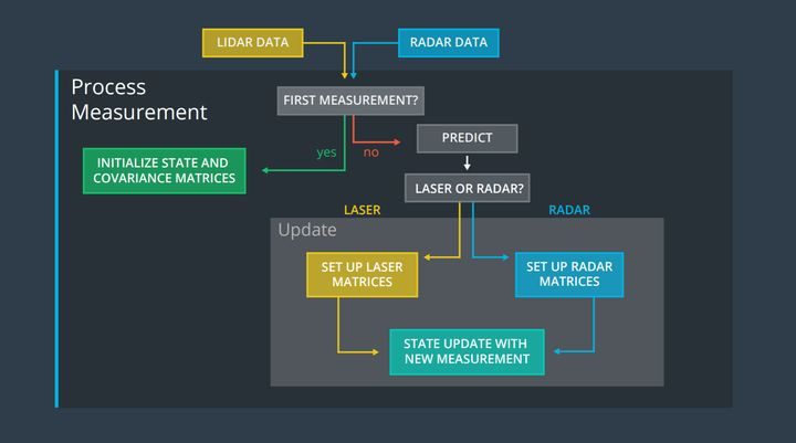
Firstly, read in sensor data. If it is the first reading, the matrices of the Kalman filter need to be initialized. If it is not the first reading, it means that the Kalman filter has completed initialization, and then we can directly conduct the state prediction and state update steps. Finally, output the fused obstacle position and velocity.
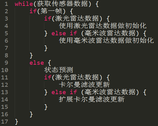
We write the above process into pseudo code to facilitate our understanding of subsequent development work.
```Translated Markdown text:
By comparing the KF and EKF code in "Introduction to Autonomous Driving Technology (Part Thirteen) | Hand in Hand to Teach You How to Write Kalman Filters" and "Introduction to Autonomous Driving Technology (Part Eighteen) | Hand in Hand to Teach You How to Write Extended Kalman Filters," we find that for the constant velocity motion model, KF and EKF have the same state prediction (Predict) process. The only difference between KF and EKF lies in the measurement update (Update) step. In the measurement update, the measurement matrix H used by KF is constant, while the measurement matrix H used by EKF is the Jacobian matrix.
Therefore, we can write KF and EKF as the same class, which has two Update functions named KFUpdate and EKFUpdate respectively. These two functions correspond to the "Kalman filter update" on line 12 and the "extended Kalman filter update" on line 15 in the pseudocode.
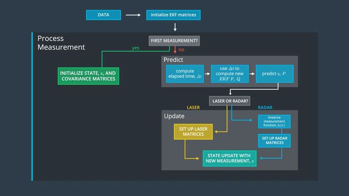
Based on the two major processes of Kalman filter prediction and measurement update, we refine the algorithmic logic as shown below.
Next, we combine the tracking algorithm codes of KF and EKF and encapsulate them in a class named KalmanFilter for convenient future calling. The rewritten KalmanFilter class is as follows:
//@ filename: /algorithims/kalman.h
#pragma once
#include "Eigen/Dense"
class KalmanFilter {
public:
KalmanFilter ();
~KalmanFilter ();
void Initialization (Eigen::VectorXd x_in);
bool IsInitialized ();
void SetF (Eigen::MatrixXd F_in);
void SetP (Eigen::MatrixXd P_in);
void SetQ (Eigen::MatrixXd Q_in);
void SetH (Eigen::MatrixXd H_in);
void SetR (Eigen::MatrixXd R_in);
void Prediction ();```
void KFUpdate (Eigen::VectorXd z);
void EKFUpdate (Eigen::VectorXd z);
Eigen::VectorXd GetX ();
private:
void CalculateJacobianMatrix ();
//flag of initialization
bool is_initialized_;
//state vector
Eigen::VectorXd x_;
//state covariance matrix
Eigen::MatrixXd P_;
//state transistion matrix
Eigen::MatrixXd F_;
//process covariance matrix
Eigen::MatrixXd Q_;
//measurement matrix
Eigen::MatrixXd H_;
//measurement covariance matrix
Eigen::MatrixXd R_;
};
//@ filename: /algorithims/kalman.cpp
#include "kalmanfilter.h"
KalmanFilter::KalmanFilter ()
{
is_initialized_ = false;
}
KalmanFilter::~KalmanFilter ()
{
}
void KalmanFilter::Initialization (Eigen::VectorXd x_in)
{
x_ = x_in;
}
bool KalmanFilter::IsInitialized ()
{
return is_initialized_;
}
void KalmanFilter::SetF (Eigen::MatrixXd F_in)
{
F_ = F_in;
}
void KalmanFilter::SetP (Eigen::MatrixXd P_in)
{
P_ = P_in;
}
cpp
void KalmanFilter::SetQ (Eigen::MatrixXd Qin)
{
Q = Q_in;
}
void KalmanFilter::SetH (Eigen::MatrixXd Hin)
{
H = H_in;
}
void KalmanFilter::SetR (Eigen::MatrixXd Rin)
{
R = R_in;
}
void KalmanFilter::Prediction ()
{
x_ = F_ * x;
Eigen::MatrixXd Ft = F.transpose ();
P_ = F_ * P_ * Ft + Q_;
}
void KalmanFilter::KFUpdate (Eigen::VectorXd z)
{
Eigen::VectorXd y = z – H_ * x;
Eigen::MatrixXd Ht = H.transpose ();
Eigen::MatrixXd S = H_ * P_ * Ht + R;
Eigen::MatrixXd Si = S.inverse ();
Eigen::MatrixXd K = P * Ht * Si;
x_ = x_ + (K * y);
int xsize = x.size ();
Eigen::MatrixXd I = Eigen::MatrixXd::Identity (xsize, xsize);
P_ = (I – K * H) * P;
}
void KalmanFilter::EKFUpdate (Eigen::VectorXd z)
{
double rho = sqrt (x(0)x(0) + x(1)x(1));
double theta = atan2 (x(1), x(0));
double rhodot = (x(0)x(2) + x(1)x(3)) /rho;
Eigen::VectorXd h = Eigen::VectorXd (3);
h << rho, theta, rhodot;
}
Eigen::VectorXd y = z - h;

CalculateJacobianMatrix ();

Eigen::MatrixXd Ht = H_.transpose ();
Eigen::MatrixXd S = H_ * P_ * Ht + R_;
Eigen::MatrixXd Si = S.inverse ();
Eigen::MatrixXd K =  P_ * Ht * Si;
x_ = x_ + (K * y);
int x_size = x_.size ();
Eigen::MatrixXd I = Eigen::MatrixXd::Identity (x_size, x_size);
P_ = (I - K * H_) * P_;
```

```
Eigen::VectorXd KalmanFilter::GetX ()
{
    return x_;
}

void KalmanFilter::CalculateJacobianMatrix ()
{
    Eigen::MatrixXd Hj (3, 4);

    //get state parameters
    float px = x_(0);
    float py = x_(1);
    float vx = x_(2);
    float vy = x_(3);

    //pre-compute a set of terms to avoid repeated calculation
    float c1 = px * px + py * py;
    float c2 = sqrt (c1);
    float c3 = (c1 * c2);

    // Check division by zero
    if (fabs (c1) < 0.0001){
        H_ = Hj;
        return;
    }

    Hj << (px/c2), (py/c2), 0, 0,
         -(py/c1), (px/c1), 0, 0,
py(vxpy – vypx)/c3, px(pxvy – pyvx)/c3, px/c2, py/c2;
H_ = Hj;
The KalmanFilter class encapsulates seven formulas of the Kalman filter, and is specifically designed for obstacle tracking. In order to make the code as decoupled and structured as possible, we create a new class called SensorFusion. The purpose of this class is to separate the **data layer** from the **algorithm layer**. Even if the interface of the data structure passed in externally changes, modifying the SensorFusion class can adapt the data without modifying the KalmanFilter algorithm, strengthening the reusability of the algorithm.
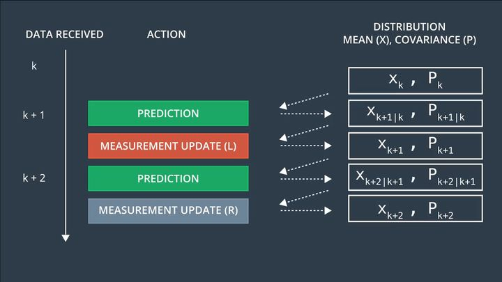
Add a function `Process()` in the `SensorFusion` class to pass in the observation values, and call the algorithm in the function `Process()`. As shown in the figure below, when laser radar data is received at time k+1, complete a prediction based on the state at time k, and then implement a measurement update (KFUpdate) based on the observation data of the laser radar at time k+1; when the millimeter-wave radar data is received at time k+2, complete a prediction based on the state at time k+1, and then implement a measurement update (EKFUpdate) based on the observation data of the millimeter-wave radar at time k+2.
Code the above process and implement it in the SensorFusion class as shown below:
cpp
//@ filename: /algorithims/sensorfusion.h
pragma once
include “interface/measurement_package.h”
include “kalmanfilter.h”
class SensorFusion {
public:
SensorFusion ();
~SensorFusion ();
void Process (MeasurementPackage measurementpack);
KalmanFilter kf;
private:
bool isinitialized;
long lasttimestamp;
}
Eigen::MatrixXd R_lidar_;
Eigen::MatrixXd R_radar_;
Eigen::MatrixXd H_lidar_;
};

//@ filename: /algorithims/sensorfusion.cpp
#include "sensorfusion.h"

SensorFusion::SensorFusion () {
    is_initialized_ = false;
    last_timestamp_ = 0.0;

    // Set Lidar's measurement matrix H_lidar_
    H_lidar_ = Eigen::MatrixXd (2, 4);
    H_lidar_ << 1, 0, 0, 0,
                0, 1, 0, 0;

    // Set R. R is provided by Sensor supplier, in sensor datasheet
    // set measurement covariance matrix
    R_lidar_ = Eigen::MatrixXd (2, 2);
    R_lidar_ << 0.0225, 0,
                0, 0.0225;

    // Measurement covariance matrix - radar
    R_radar_ = Eigen::MatrixXd (3, 3);
    R_radar_ << 0.09, 0, 0,
                0, 0.0009, 0,
                0, 0, 0.09;
}

SensorFusion::~SensorFusion () {

}

void SensorFusion::Process (MeasurementPackage measurement_pack) {
    // The first data frame is used to initialize the Kalman filter
    if (!is_initialized_) {
```
```
`Eigen::Vector4d x;`
if (measurement_pack.sensor_type_ == MeasurementPackage::LASER) {
    // If the first frame of data is from a laser measurement, there is no velocity information available. Therefore, set the velocity components to 0
    x << measurement_pack.raw_measurements_[0], measurement_pack.raw_measurements_[1], 0, 0;
} else if (measurement_pack.sensor_type_ == MeasurementPackage::RADAR) {
    // If the first frame of data is from a radar measurement, position and velocity components can be calculated from the trigonometric functions.
    float rho = measurement_pack.raw_measurements_[0];
    float phi = measurement_pack.raw_measurements_[1];
    float rho_dot = measurement_pack.raw_measurements_[2];
    float position_x = rho * cos (phi);
    if (position_x < 0.0001) {
        position_x = 0.0001;
    }
    float position_y = rho * sin (phi);
    if (position_y < 0.0001) {
        position_y = 0.0001;
    }
    float velocity_x = rho_dot * cos (phi);
    float velocity_y = rho_dot * sin (phi);
}
markdown
 x << position_x, position_y, velocity_x , velocity_y;
}

// Avoids 0 as the denominator in calculations
if (fabs(x(0)) < 0.001) {
    x(0) = 0.001;
}
if (fabs(x(1)) < 0.001) {
    x(1) = 0.001;
}
// Initialize the Kalman filter
kf_.Initialization(x);

// Set the covariance matrix P
Eigen::MatrixXd P = Eigen::MatrixXd(4, 4);
P << 1.0, 0.0, 0.0, 0.0,
     0.0, 1.0, 0.0, 0.0,
     0.0, 0.0, 1000.0, 0.0,
     0.0, 0.0, 0.0, 1000.0;
kf_.SetP(P);

// Set the process noise Q
Eigen::MatrixXd Q = Eigen::MatrixXd(4, 4);
Q << 1.0, 0.0, 0.0, 0.0,
     0.0, 1.0, 0.0, 0.0,
     0.0, 0.0, 1.0, 0.0,
     0.0, 0.0, 0.0, 1.0;
kf_.SetQ(Q);

// Store the timestamp of the first frame for the use of the next data frame
last_timestamp_ = measurement_pack.timestamp_;
is_initialized_ = true;
return;
}

// Calculate the time difference between the two frames. The timestamp in the data packet is in microseconds, divide by 1e6, and convert to seconds.
“`markdown
double deltat = (measurementpack.timestamp_ – lasttimestamp) / 1000000.0; //unit : s
lasttimestamp = measurementpack.timestamp;
Eigen::MatrixXd F = Eigen::MatrixXd(4, 4);
F << 1.0, 0.0, deltat, 0.0,
0.0, 1.0, 0.0, deltat,
0.0, 0.0, 1.0, 0.0,
0.0, 0.0, 0.0, 1.0;
kf_.SetF(F);
kf_.Prediction();
if (measurementpack.sensortype_ == MeasurementPackage::LASER) {
kf.SetH(Hlidar);
kf.SetR(Rlidar);
kf.KFUpdate(measurementpack.rawmeasurements);
} else if (measurementpack.sensortype_ == MeasurementPackage::RADAR) {
kf.SetR(Rradar_);
<!-- Jacobian 矩阵 Hj 的运算已包含在 EKFUpdate 中 -->
kf_.EKFUpdate(measurement_pack.raw_measurements_);
}
### Sensor Fusion Result Output

After completing the sensor data reading and fusion algorithm writing, we combine them in main.cpp, outputting the obstacle fusion results of each frame.
cpp
//@ filename: main.cpp
include
include
include
include
include
“`# Set the path of input data for radar and lidar
std::string inputfilename = “../data/sample-laser-radar-measurement-data-2.txt”;
Open the file and print an error message if failing
std::ifstream inputfile (inputfilename.cstr (), std::ifstream::in);
if (!inputfile.isopen ()) {
std::cout << “Failed to open file named :” << inputfilename << std::endl;
return -1;
}
Allocate memory for measurementpacklist and groundtruthpacklist
measurementpacklist: contains the actual measurements from radar and lidar, with measurement values and timestamps, as input to the fusion algorithm.
groundtruthpacklist: contains the ground truth about object positions at each measurement. Used to evaluate the fusion algorithm’s output against the ground truth.
std::vector
std::vector
Use a while loop to read in all the radar measurements and ground truth into memory, and store them in measurementpacklist and groundtruthpacklist.“`
// Store radar & lidar data into memory
std::string line;
while (getline (inputfile, line)) {
std::string sensortype;
MeasurementPackage measpackage;
GroundTruthPackage gtpackage;
std::istringstream iss (line);
long long timestamp;
// Reads first element from the current line. L stands for Lidar. R stands for Radar.
iss >> sensortype;
if (sensortype.compare (“L”) == 0) {
// Lidar data
// 2nd element is x; 3rd element is y; 4th element is timestamp (nano second)
measpackage.sensortype_ = MeasurementPackage::LASER;
measpackage.rawmeasurements_ = Eigen::VectorXd (2);
float x;
float y;
iss >> x;
iss >> y;
measpackage.rawmeasurements_ << x, y;
iss >> timestamp;
measpackage.timestamp = timestamp;
measurement_pack_list.push_back (meas_package);
        } else if (sensor_type.compare ("R") == 0) {

<!-- Radar data in millimeter waves -->

<!-- 2nd element is pho; 3rd element is phi; 4th element is pho_dot; 5th element is timestamp (nano second) -->

            meas_package.sensor_type_ = MeasurementPackage::RADAR;
            meas_package.raw_measurements_ = Eigen::VectorXd (3);
            float rho;
            float phi;
            float rho_dot;
            iss >> rho;
            iss >> phi;
            iss >> rho_dot;
            meas_package.raw_measurements_ << rho, phi, rho_dot;
            iss >> timestamp;
            meas_package.timestamp_ = timestamp;
            measurement_pack_list.push_back (meas_package);
        }

<!-- The last four elements of the current row are the true distances in x and y, and the true speeds in the x and y directions respectively. -->

<!-- read ground truth data to compare later -->
        float x_gt;
        float y_gt;
        float vx_gt;
float vygt;
iss >> xgt;
iss >> ygt;
iss >> vxgt;
iss >> vygt;
gtpackage.gtvalues = Eigen::VectorXd(4);
gtpackage.gtvalues_ << xgt, ygt, vxgt, vygt;
groundtruthpacklist.pushback(gtpackage);
std::cout << “Success to load data.” << std::endl;
// Deploy tracking algorithm
SensorFusion fuser;
for (sizet i = 0; i < measurementpacklist.size(); ++i) {
fuser.Process(measurementpacklist[i]);
Eigen::Vector4d xout = fuser.kf_.GetX();
// Output location after tracking
std::cout << "x" << x_out(0)
    << "y" << x_out(1)
    << "vx" << x_out(2)
    << "vy" << x_out(3)
    << std::endl;
}
“`
Deploy the tracking algorithm and plot the fusion result and ground truth in the same coordinate system, as shown below:
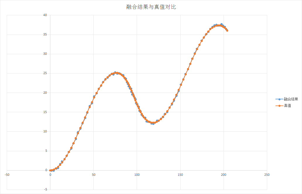 The fusion results are consistent with the truth, but only qualitative analysis is conducted, lacking quantitative description. Later in the course, a quantitative analysis method is introduced – Root Mean Squared Error (RMSE), which calculates the square root of the mean squared deviations of predicted values from true values divided by the number of observations n. The calculation formula is shown as follows:
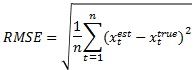
Calculate the RMSE for x, y, vx, and vy, and smaller RMSE values indicate closer results to the truth and better tracking performance.
Udacity’s Self-Driving Car Engineer Program provides a convenient visualization tool in the course to real-time display the tracking state of obstacles and the value of RMSE. The red and blue dots in the video represent the measurement positions of radar and lidar, respectively, and the green dot represents the output result after multi-sensor fusion, with the true value being the position of the car.
Multi-sensor Fusion
Conclusion
Above are the technical principles and programming ideas of multi-sensor fusion. The complete code and the method of building a Linux open environment can be obtained by following the WeChat public account “Autonomous Driving Knowledge Base” and replying “Sensor Fusion”.As an introductory course, this sharing only introduced the fusion of LiDAR and mmWave radar for single obstacle detection. In the development of practical engineering, multi-sensor fusion algorithm engineers not only need to master the theory and coding of fusion algorithms, but also learn about the data characteristics of different sensors (such as LiDAR, mmWave radar, cameras, etc.) and the corresponding obstacle detection algorithms, in order to be proficient in various sensors.
If you want to delve deeper into the technology of multi-sensor data processing and fusion, you can learn about the Udacity Sensor Fusion Nanodegree program! Here is an invitation code worth ¥320: 50C3D1EA.
Alright (^o^)/~, this sharing about sensor fusion technology ends here. If you have any questions, feel free to discuss with me in the comments section.
This article is a translation by ChatGPT of a Chinese report from 42HOW. If you have any questions about it, please email bd@42how.com.