Introduction
In the previous article “Introduction to Autonomous Driving Technology (16) | Introduction to Deep Learning: Traffic Sign Classification,” I used traffic sign classification as an example to introduce the theoretical knowledge about neural networks involved in deep learning. This includes the parameters of neural networks, the principle of backpropagation, and the difference between training sets, validation sets, and test sets. By optimizing the classical image classification network LeNet-5, we completed the classification of traffic signs.
In this sharing, I will take Udacity’s Self-Driving Car Engineer Nanodegree Program’s behavior cloning project as an example to introduce the application of deep learning in end-to-end autonomous driving control. End-to-end means from the image end to the control end, that is, the technique of inputting the image results taken by the camera into the neural network and directly outputting information such as steering wheel angle, throttle, and brake pedal opening of the autonomous vehicle.
Main Body
When using deep learning to “clone” the behavior of autonomous vehicles “end-to-end,” the first problem encountered is the lack of data. Currently, most of the data sets in the field of computer vision are collected on vehicles and labeled, but the corresponding data sets do not include data related to vehicle control, such as steering wheel angle and vehicle speed.
Fortunately, the open course MIT 6.S094 provides some Tesla driving data sets, which include images from the Tesla’s front camera and the corresponding steering wheel angle for each frame. Although the data is limited, we can at least try to build a model to achieve end-to-end autonomous vehicle control. Udacity has published an article “A Beginner’s Guide to Autonomous Vehicles–Teaching Tesla to Drive Like Humans” that uses this data set to predict the steering wheel angle “end-to-end.” The data and code can be found here.
The result of steering wheel angle prediction is shown in the lower right corner of the figure below. The blue line is the true value of the steering wheel angle, and the pink line is the predicted value of the steering wheel angle based on the current image.
“>
图片出处:https://github.com/nd009/capstone/tree/master/deep_tesla
The Tesla Dataset has two major shortcomings. First, the amount of data is insufficient, and the network model trained is not sufficiently generalized. Second, after predicting the steering angle, it can only achieve a simple comparison between the predicted value and the true value, and cannot be used as an input to control the vehicle’s chassis, which is commonly known in the industry as the “closed loop” that cannot be controlled.
Self-driving Simulator
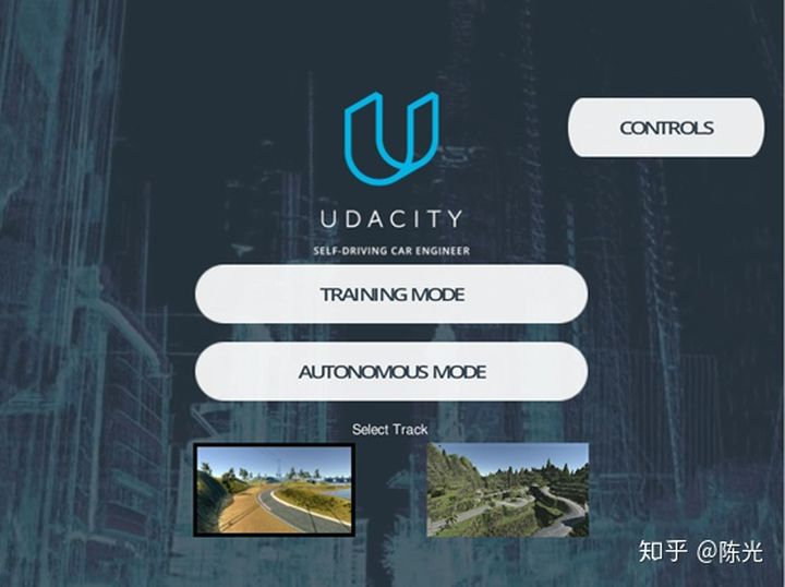
To solve the “closed loop” problem of end-to-end, Udacity’s instructors of the self-driving engineer program have designed a multi-platform (Mac, Linux, Windows) simulator, self-driving-car-sim, which not only can collect data, but also can implement end-to-end steering control of autonomous vehicles by importing trained deep learning models.
The simulator self-driving-car-sim contains two modes — Training Mode and Autonomous Mode.
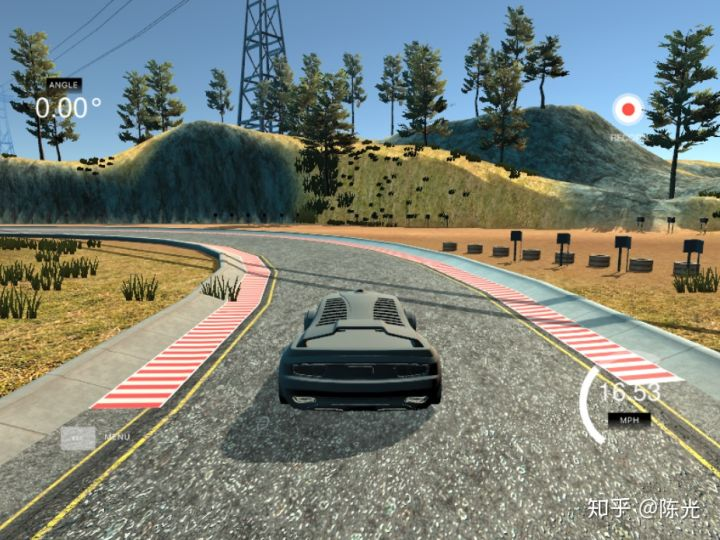
The Training Mode, which can also be understood as the data collection mode. Click on the record button displayed in the figure to control the car’s driving by using the arrow keys. Control your car to drive a certain distance, and then click again. The simulator will record and store the data of the road you just drove manually.
The stored data contains a table, and each row of the table records the storage path of the image taken by the on-board camera and the control signal of the vehicle at the time of shooting. There are three on-board cameras installed on the car, which are respectively installed on the left, center and right of the car, as shown in the figure below.
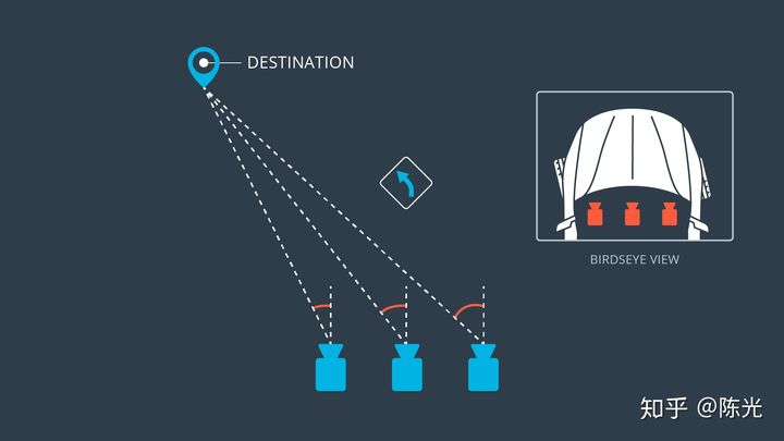
Image source: Udacity self-driving engineer program
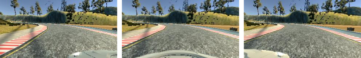
Each group (frame) of data will contain images from three viewpoints, steering angle, and vehicle speed. As shown in the figure below, the road images from the three viewpoints can be judged by the position of the car’s hood.
“`### Data Collection and Preprocessing
The route provided by the simulator forms a loop, where most of the segments turn left when controlling the vehicle. Recording data only in one turning direction would lead to a model that tends to turn left regardless of road conditions, which is not what we want. To avoid this, we need to record driving data in both clockwise and counterclockwise directions to make the trained model more generalized.
In addition to recording data in both directions, we can also use data augmentation techniques to increase the diversity of data, as mentioned in the previous section. The most direct way to augment data in this project is to mirror the images horizontally, and then add a negative sign to the corresponding steering angle. This will double the size of the dataset.
Apart from the center camera installed on the vehicle, the cameras on the left and right sides can also provide useful data. First, using the data from both sides can double the dataset again. Second, since the side cameras are closer to the edge of the road, they can teach the network how to steer back to the center of the road when the vehicle starts to deviate. We just need to adjust the corresponding steering angle by adding or subtracting a correction value when using this data.
After all of these steps, the dataset size will increase by a factor of 6. Next, we need to preprocess the data.
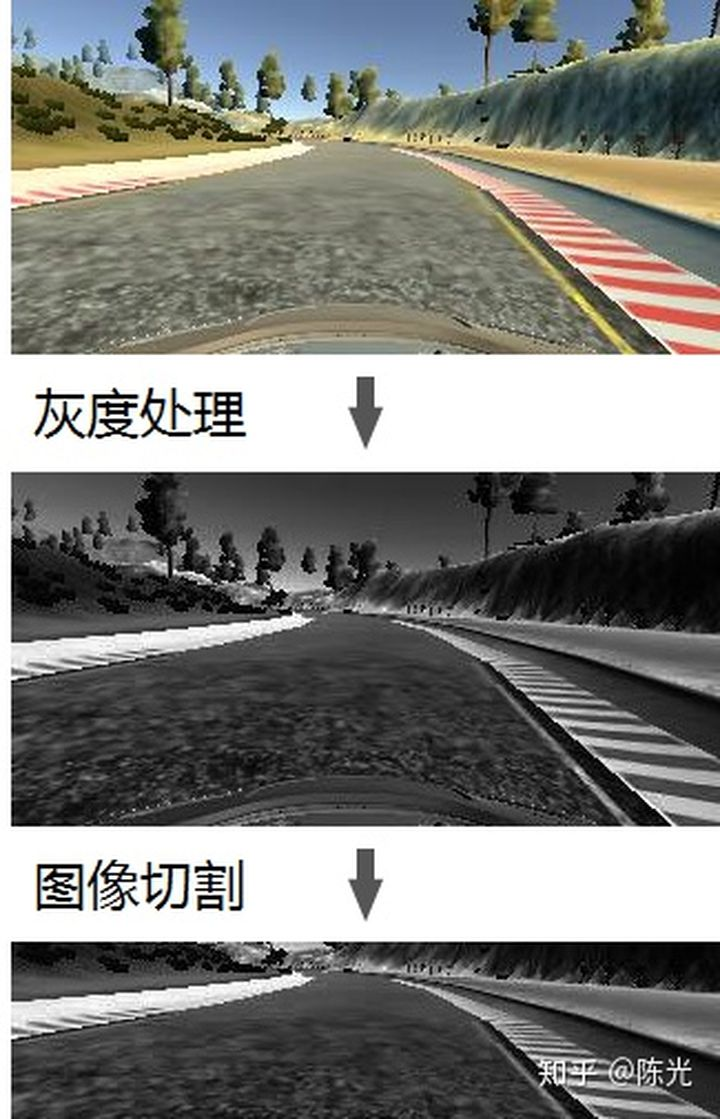
As we can see from the images, the color information does not have a significant impact on the steering angle of the vehicle. Even grayscale images can be used to steer the car. Therefore, we will convert the color images to grayscale to reduce the complexity of the input images to the model. Since the road shape affects the steering angle, the sky and trees in the image are not the focus of the model. We can crop the sky and trees to make the road occupy more of the image. The preprocessing steps for the images are shown in the following figure:
After completing the data collection and preprocessing process, let’s start building the end-to-end network model.
End-to-End Network Model
In the field of deep learning, researchers usually don’t build neural networks from scratch. Building a neural network from scratch requires designing the network architecture and conducting a lot of training and testing to prove that the network is effective, which can be very time-consuming and challenging. To speed up the work, researchers usually start with pre-trained networks and modify or fine-tune them for their specific tasks. This type of modification of a mature network is called ” transfer learning “.
In other words, we can borrow from others’ networks to solve similar problems.The autonomous vehicle team at NVIDIA proposed a network in August 2016, specialized for achieving end-to-end autonomous driving, which they also used for real-car training. This network can serve as a reference for us to learn from. The structure of the model is shown below:
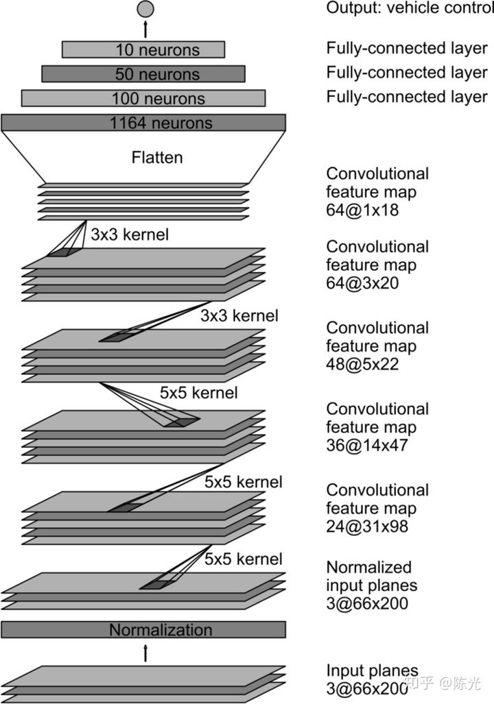
Image source: https://devblogs.nvidia.com/deep-learning-self-driving-cars/
From bottom to top, the network contains a normalization layer, followed by 5 convolutional layers, connected to 4 fully connected layers, and finally outputs the vehicle’s control signal, which can be the steering wheel angle or the speed.
We can quickly build this network using TensorFlow’s Keras library as shown below:
from keras.models import Sequential, Model
from keras.layers import Lambda, Input, Flatten, Dense, Cropping2D, Convolution2D

model = Sequential ()
#normalize image
model.add (Lambda (lambda x: x / 127.5 - 1.0, input_shape=(66, 200, 3)))
#convolution layer
model.add (Convolution2D (24,5,5,strides=(2,2), activation="relu"))
model.add (Convolution2D (36,5,5,strides=(2,2), activation="relu"))
model.add (Convolution2D (48,5,5,strides=(2,2), activation="relu"))
model.add (Convolution2D (64,3,3, activation="relu"))
model.add (Convolution2D (64,3,3, activation="relu"))
#flatten layer
model.add (Flatten ())
model.add (Dense (100))
“`markdown
model.add(Dense(50))
model.add(Dense(10))
model.add(Dense(1))
Due to the difference in image size between our images and the size used by the model, as well as the preprocessing steps performed on the images (grayscale conversion and cropping), some modifications need to be made to the model. The modified model is shown below:
from keras.models import Sequential, Model
from keras.layers import Lambda, Input, Flatten, Dense, Cropping2D, Convolution2D
inputshape = (160, 320, 3)
outputshape = (160, 320, 1)
normalized_shape = (80, 320, 1)
model = Sequential()
User-defined grayscale function
model.add(Lambda(color2gray, inputshape=inputshape, outputshape=outputshape))
Cropping
model.add(Cropping2D(cropping=((50,30), (0,0))))
Normalizing image
model.add(Lambda(lambda x: x / 127.5 – 1.0, inputshape=normalizedshape))
Convolution layer
model.add(Convolution2D(24, 5, 5, strides=(2,2), activation=”relu”))
model.add(Convolution2D(36, 5, 5, strides=(2,2), activation=”relu”))
model.add(Convolution2D(48, 5, 5, strides=(2,2), activation=”relu”))
model.add(Convolution2D(64, 3, 3, activation=”relu”))
model.add(Convolution2D(64, 3, 3, activation=”relu”))
Flatten layer
model.add(Flatten())
“““
model.add(Flatten())
model.add(Dense(100))
model.add(Dense(50))
model.add(Dense(10))
model.add(Dense(1))
After building the model, we select 80% of the previous data as the training set and the remaining 20% as the validation set to start training the model.
### Overfitting Problem
After training the model with the above data and network, when applying the model to the simulator to let the car drive automatically, it will be found that the car will run out of the track after a period of time. At this time, we encounter a problem frequently encountered in the field of deep learning - overfitting.
The most obvious feature of an overfitted model is that it performs perfectly on the training set, but poorly on the validation set. If the model performs poorly on the validation set, when applying the model to actual scenarios, it will not perform well.
Next, I will explain the overfitting phenomenon with a simple example, and discuss how to solve the problem when the model is overfitted.
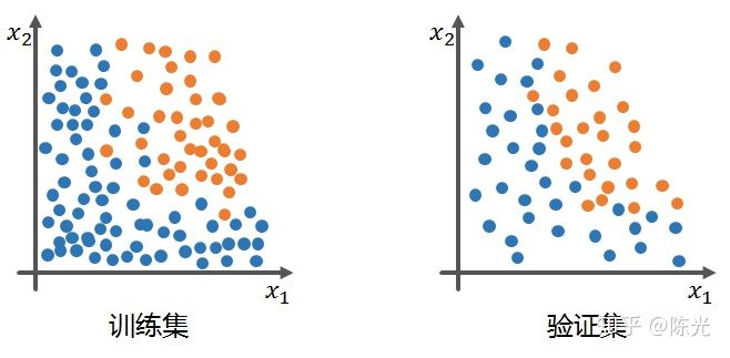
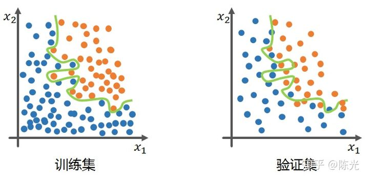
Assume that our training and validation sets are blue and orange points below, we need to train a model that can distinguish different colored points.
The ideal model trained on the training set should be able to achieve high accuracy in the classification effect in the training set, and when applied to the validation set, it should perform well. The green line in the figure below shows the ideal model trained on the training set.
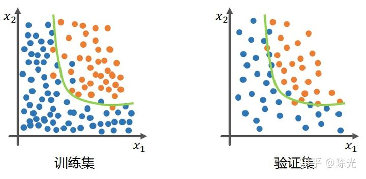
An overfitted model has an obvious feature, which is that it can achieve high accuracy on the training set, but once the model is applied to the validation set, the effect is very poor, as shown by the green line in the figure below, which is a typical overfitted model. The overfitted model performs well on the training set, but this performance is not general enough, resulting in a low accuracy when applied to the validation set.
To solve the overfitting problem of the end-to-end autonomous car control model, the teachers at Udacity propose four solutions:
1. Add dropout layers to the network
2. Add pooling layers to the network
3. Use fewer convolutional or fully connected layers
4. Collect more data or use data augmentation to enrich the dataset.The network architecture of the convolutional part remains unchanged in order to avoid significant discrepancies with the original model. However, in the modified model, we added a Dropout layer and fine-tuned the fully connected layer to reduce overfitting. After multiple trials, we found a network model that meets the project requirements. The modified model is shown below:
python
from keras.models import Sequential, Model
from keras.layers import Lambda, Input, Flatten, Dense, Cropping2D, Convolution2D
inputshape = (160, 320, 3)
ouputshape = (160, 320, 1)
normalized_shape = (80, 320, 1)
model = Sequential ()
user defined grayscale function
model.add (Lambda (color2gray, inputshape = inputshape, outputshape= ouputshape))
cropping
model.add (Cropping2D (cropping=((50,30), (0,0))))
normalize image
model.add (Lambda (lambda x: x / 127.5 – 1.0, inputshape=normalizedshape))
convolution layer
model.add (Convolution2D (24,5,5,strides=(2,2), activation=”relu”))
model.add (Convolution2D (36,5,5,strides=(2,2), activation=”relu”))
model.add (Convolution2D (48,5,5,strides=(2,2), activation=”relu”))
model.add (Convolution2D (64,3,3, activation=”relu”))
model.add (Convolution2D (64,3,3, activation=”relu”))
flatten layer
model.add (Flatten ())
```markdown
model.add(Dropout(0.5)) # reduce overfitting
model.add(Dense(180, activation="relu"))
model.add(Dense(60))
model.add(Dense(10, activation="relu"))
model.add(Dense(1))
### Video of Results

After training the model with the augmented training set and modified network, follow the instructions of the self-driving car clone project to run the model and enter the self-driving mode of the simulator.

Check out the results of the final end-to-end autonomous driving of the self-driving car in the video below.
<video controls class="w-full" preload="metadata" poster="https://upload.42how.com/article/image_20210302003836.png">
<source src="https://vdn.vzuu.com/SD/v3_fb4a0dcc-50ae-11e9-8de2-0a580a405e32.mp4?disable_local_cache=1&auth_key=1614620246-0-0-6ee8cc9c6e6f256bcdf7d54b98b58964&f=mp4&bu=http-com&expiration=1614620246&v=ali">
</video>


End-to-End Autonomous Driving of the Self-Driving Car
From the final "closed-loop" results, we can see that the self-driving car has indeed learned end-to-end autonomous driving. There may be some noticeable turning delays in certain areas, which may require more data or better models to solve these problems.

### Conclusion

This is the entire content of "Introduction to Autonomous Driving Technology (Part 17) - Advanced Deep Learning in Self-Driving Car Behavior Clone." In this sharing, I introduced the self-driving car simulator provided by Udacity, completed data collection using the simulator, followed by augmentation and preprocessing of the collected data. After modifying the end-to-end network proposed by the Nvidia self-driving car team, the model was trained and the project requirements were completed.

Through this sharing, we can see that with enough data, deep learning can not only solve the problem of traffic sign classification but also be used to solve more complex issues, such as self-driving car behavior cloning.
The behavior cloning technology for end-to-end driving is currently limited to laboratory experiments, and it is not yet widely used in actual road tests. This is because any decision involving the control layer of an autonomous vehicle must be traceable, and deep learning, as an untraceable “black box,” even if it performs well in the laboratory environment, engineers dare not use it recklessly in road tests.
That’s all for this sharing (^o^)/~, see you in the next issue~
This article is a translation by ChatGPT of a Chinese report from 42HOW. If you have any questions about it, please email bd@42how.com.